Adaptive Kinetic Monte Carlo Simulation of Pt Island Ripening
Version: 2017
This tutorial is on the use of the Adaptive Kinetic Monte Carlo (AKMC) method. It will cover setting up a simulation to model Pt island ripening on a Pt(111) surface, how to implement the Morse potential, and how to analyze the results. For more information on the AKMC method, you may look at the following tutorials: AKMC Simulation of Pt on Pt(100) and Modeling Vacancy Diffusion in SiGe alloy.
Introduction
In this tutorial we will model island ripening of Pt adatoms on a Pt(111) surface at 300 K using the Adaptive Kinetic Monte Carlo (AKMC) method. The initial surface will have seven adatoms and the most stable structure is a compact heptamer island. The atomic interactions will be modeled using a simple Morse potential to allow us to compare our results to a published benchmark study [1]. The use of the Morse potential also allow us to showcase the use of AKMC without resorting to computationally expensive DFT calculations, but it is not expected to directly reproduce a particular experimental result.
Creating the initial configuration
The initial configuration will be a 4 layer p (6x6)-Pt(111) slab with seven adatoms occupying three-fold hollow sites.
Open the
 Builder.
Import the Pt fcc bulk configuration by clicking on and search for Platinum.
The Pt primitive cell will appear in the Stash.
Click on .
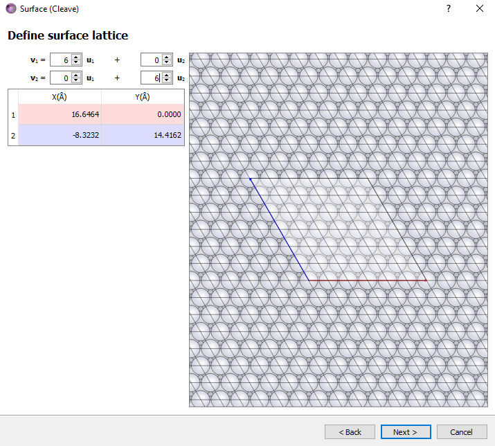
In the new window, choose the (111) Miller indices.
Define the p (6x6) surface unit cell.
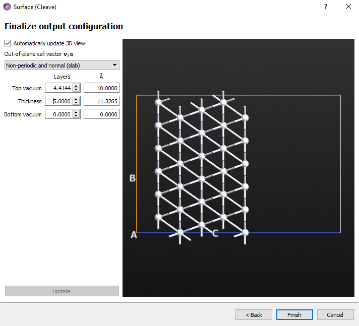
Choose the Non-periodic and normal (slab) option and a thickness of 5 layers. Click Finish button.
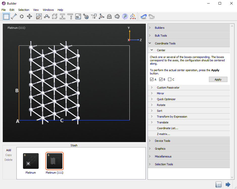
Click on and select the A and B axes and click the Apply button.
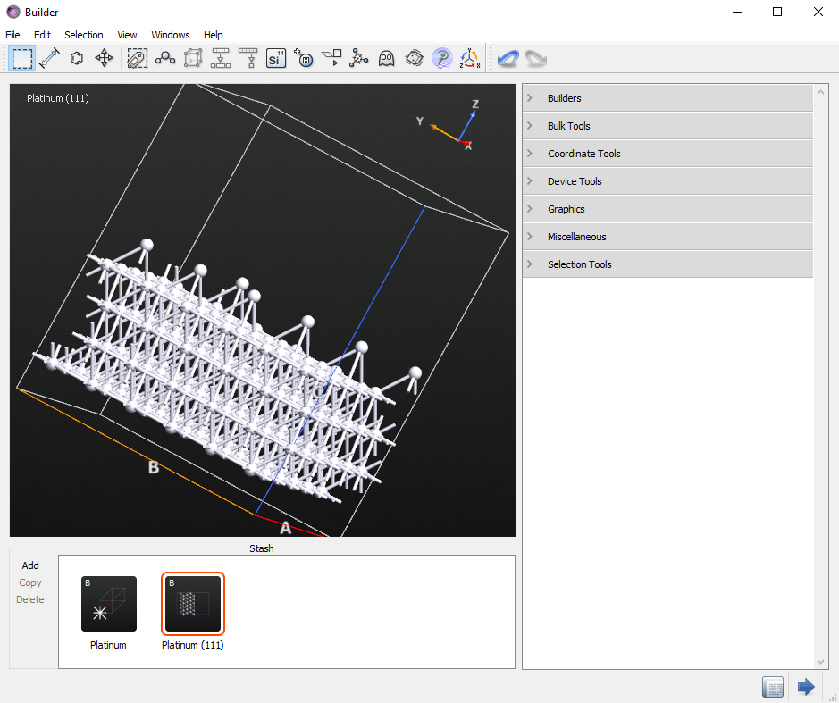
Select the whole top layer.
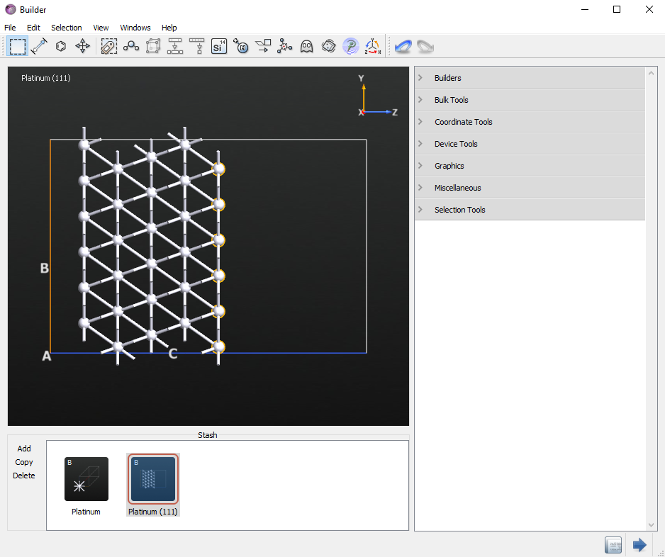
Un-select seven non-contiguous atoms holding the
shiftkey on your keyboard and then press thedelkey to remove the selected atoms. There should now be seven adatoms. It should look similar to the image below.
Send the configuration to the Script Generator by clicking the
 or dragging the structure onto the
  Scripter.
For now, do not add a calculator block. Since we are using a Morse potential, we will specify the calculator later. The parameters for the Morse potential were originally fitted to model bulk Pt and are the same as used in [1].
Add an
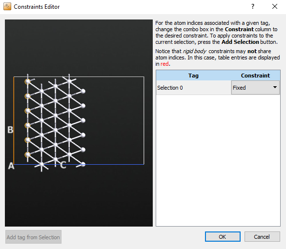
 block and double-click it. Set the Force tolerance to 0.01 eV/Å. Then click Add Constraints and select the bottom row of atoms, click Add tag from Selection, and then set the Constraint to Fixed.
Change the Default output file to
initial.hdf5.Send the script to the Editor.
We now need to define the Morse calculator. Insert the following code above the call to OptimizeGeometry:
morse_potential.py
potentialSet = TremoloXPotentialSet(name='Pt-Morse')
potentialSet.addParticleType(ParticleType.fromElement(Platinum))
potentialSet.addPotential(MorsePotential(
    'Pt',
    'Pt',
    r_0=2.897*Angstrom,
    k=1.6047*Angstrom**-1,
    E_0=0.7102*eV,
    r_i=6.5*Angstrom,
    r_cut=9.5*Angstrom)
)
calculator = TremoloXCalculator(parameters=potentialSet)
bulk_configuration.setCalculator(calculator)
Now save the script as
initial.pyor download theinitial.pyand send it to the Job Manager and run it.
The optimized geometry can now be selected on the LabFloor and visualized in the Viewer. It may be useful to click on Properties in the right-hand panel and tweak the way the atoms are rendered to more easily distinguish the adatoms from the bulk atoms. In the image below, the atoms are rendered as covalent radius spheres and the adatoms are in a darker gray than the bulk Pt.
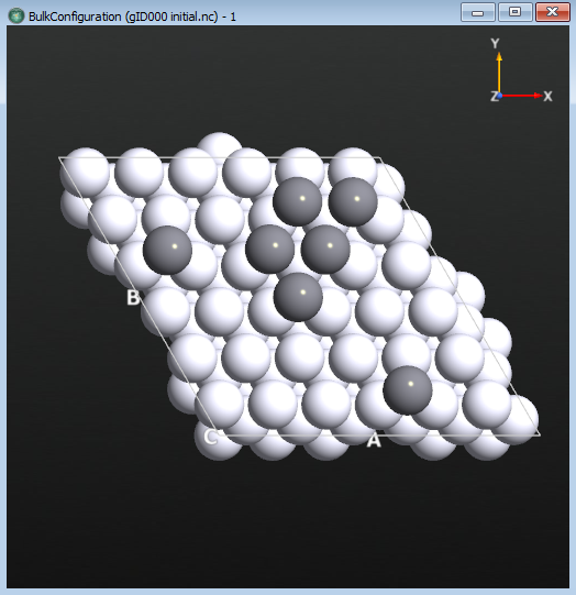
Tip
If you wish to re-create the above figure, you can do the following: Select the file initial.hdf5 file on the LabFloor. Click the Viewer on the right-hand panel. Open the Properties window. Select the Covalent option under Atoms and check Wrap atoms under Bulk. The atoms are now shown as balls with their covalent radius. Choose the top 7 Pt atoms and then change to another color (here we chose gray). Now you can distinguish the 7 adatoms on the Pt surface.
Setting up the AKMC Simulation
We will now set up and run the AKMC simulation. The goal is to determine the time required to form a compact heptamer island at 300 K.
Now that you have an optimized initial structure, you can run the AKMC simulation. Drag initial.hdf5 from the main QuantumATK window to the Scripter.
Starting from ATK 2017, AdaptiveKineticMonteCarlo is implemented in the Scripter.
Note
If you have an older version, you can download the script adding_akmc.py and append the contents in the  Editor instead of following the steps below. Instead, go to the next section: Adding the calculator
We use the Morse potential which is the same as used in [1]. After setting up the AKMC simulation, we will add the Morse Potential calculator in the editor in the next section.
In the Scripter, add an block.
Double click the
AdaptiveKineticMonteCarlo block.Go to the Optimization tab, and click on the Atomic Constraint Editor to add a constraint.
Select the bottom layer to be constrained, as in the initial optimization, and press the Add tag from Selection button. Change to the Fixed constraint. This will remove the red-colored warning.
In the Kinetic Monte Carlo tab, set the value to 20 in the Superbasin creation threshold.
For HTST Prefactor, we use a fixed Prefactor value of 1013 s-1 because it does not change much from one reaction to another.
Note
For most solid-state systems, the prefactor is not important to calculate directly (and it is expensive to do so). The primary difference between different reaction mechanisms is the size of the energy barrier. In the referenced simulation we are comparing against, this step was skipped.
In the Saddle Search settings, set the number of searches to 200.
Change the Default output file name to
akmc.hdf5and go to the Editor by clicking the icon.
Adding the calculator
Now we need to add the Morse potential calculator above the AKMC calculation in the Editor using the script morse_potential.py.
# Morse-potential
potentialSet = TremoloXPotentialSet(name='Pt-Morse')
potentialSet.addParticleType(ParticleType.fromElement(Platinum))
potentialSet.addPotential(MorsePotential(
    'Pt',
    'Pt',
    r_0=2.897*Angstrom,
    k=1.6047*Angstrom**-1,
    E_0=0.7102*eV,
    r_i=6.5*Angstrom,
    r_cut=9.5*Angstrom)
)
calculator = TremoloXCalculator(parameters=potentialSet)
bulk_configuration.setCalculator(calculator)

# -------------------------------------------------------------
# Adaptive Kinetic Monte Carlo
# -------------------------------------------------------------
htst_parameters = HTSTParameters(
    assumed_prefactor=1e+13*1/Second,
    )

if os.path.isfile('akmc_markov_chain.hdf5'):
    markov_chain = nlread('akmc_markov_chain.hdf5')[-1]
else:
    markov_chain = MarkovChain(
        configuration=bulk_configuration,
        configuration_energy=TotalEnergy(bulk_configuration).evaluate(),
        )

if os.path.isfile('akmc_kmc.hdf5'):
    kmc = nlread('akmc_kmc.hdf5')[-1]
else:
    kmc = None

constraints = [ 0,  1,  2,  3,  4,  5,  6,  7,  8,  9, 10, 11, 12,
               13, 14, 15, 16, 17, 18, 19, 20, 21, 22, 23, 24, 25,
               26, 27, 28, 29, 30, 31, 32, 33, 34, 35]

akmc = AdaptiveKineticMonteCarlo(
    markov_chain=markov_chain,
    kmc_temperature=300.0*Kelvin,
    md_temperature=2000.0*Kelvin,
    calculator=bulk_configuration.calculator(),
    kmc=kmc,
    superbasin_threshold=20,
    htst_parameters=htst_parameters,
    constraints=constraints,
    confidence=0.99,
    filename_prefix='akmc',
    )

akmc.run(max_searches=200, max_kmc_steps=10000)
You can also download the input file akmc.py to start the run for the AKMC simulation.
Running the Simulation
This script will run 200 saddle searches each time it is called. The first time the script is run, it creates a new AKMC simulation, while subsequent runs resume the simulation. Each saddle search takes about 15 seconds. So, in serial, 200 saddle searches will take under 1 hour to complete. The calculation can also be run in parallel using MPI, but note that you need at least 3 processes to get a speed-up. The goal of this simulation is to find the time it takes to form a compact heptamer (7 atom) island. This is the lowest energy configuration of the system. The AKMC script will have to be run several times to reach this point. After each run, you should follow the analysis below to monitor the progress of the simulation.
Note
You will probably need to run more searches to find a heptamer island with the AKMC simulation. If you do not find it within 200 searches, you can restart the simulation to search for more saddle points by using the files: akmc_markov_chain.hdf5 and akmc_kmc.hdf5, which the script is set up to do automatically. Here we ran it again up to 1000 searches.
Analyzing the AKMC Simulation
Since AKMC simulations are stochastic, your results will be slightly different from what is shown here. You can download the current results for the same analysis. akmc_log.hdf5, akmc_markov_chain.hdf5 and akmc_kmc.hdf5.
There are three output files to examine: akmc_log.hdf5, akmc_markov_chain.hdf5 and akmc_kmc.hdf5. The akmc_log.hdf5 file contains information about the results of each saddle search. If there are errors they will be reported here. The file akmc_markov_chain.hdf5 contains the energies and geometries of the different configurations and how the different configurations are connected through saddle points and their energy barriers. It also contains the data needed to compute rate constants using harmonic transition state theory. The file akmc_kmc.hdf5 stores the Kinetic Monte Carlo simulation data. This includes the current state identifier and the simulation time.
AKMC Log File
The log file should be looked at first to make sure that the simulation ran correctly. Below is an example of what the log file will look like. The log file can be viewed by clicking on the akmc_log.hdf5 file on the LabFloor and clicking the Text Representation… button in the panel on the right.
The first column shows the state id number that is used to identify each configuration in the Markov Chain. The second column shows the search number, which is a unique identifier for each saddle search. The third column shows the confidence estimate, which is a measure of the probability that all relevant saddle points have been found in that state. Saddle searches are run in each until the confidence exceeds the chosen threshold passed to the AKMC simulation. In the log file below, you can see that the initial state 0 is visited until the confidence meets 0.99, then the next state 2 is reached.
The fifth column contains a message about the saddle search. The message found new state represents a new reaction mechanism being discovered, while the message Found saddle connecting to state i again represents state i having been found again. In the state id 0, there are 7 Found new state and several Found saddle connecting to state i again. There is only one search that ended in an error in this example: search number 17. In this search a new saddle point was found, but it does not connect back to the current state. This means it is a saddle point that describes a reaction between two different states. This is expected to happen sometimes, but if a large number of the saddle searches have this message, then it probably means that the MD temperature is too high.
# Item:  0
# File:  C:\tutorial\akmc_log.nc
# Title: akmc_log.nc - gID000
# Type:  AKMCLog
state id search number confidence  message
       0             0   0.000000  Found new state
       0             1   0.000000  Found new state
       0             2   0.000000  Found new state
       0             3   0.000000  Found new state
       0             4   0.655097  Found saddle connecting to state 2 again
       0             5   0.801496  Found saddle connecting to state 4 again
       0             6   0.866310  Found saddle connecting to state 2 again
       0             7   0.927713  Found saddle connecting to state 1 again
       0             8   0.866170  Found new state
       0             9   0.507710  Found new state
       0            10   0.520759  Found saddle connecting to state 2 again
       0            11   0.878596  Found saddle connecting to state 6 again
       0            12   0.914000  Found saddle connecting to state 6 again
       0            13   0.918800  Found saddle connecting to state 2 again
       0            14   0.931824  Found saddle connecting to state 6 again
       0            15   0.933590  Found saddle connecting to state 2 again
       0            16   0.854401  Found new state
       0            17   0.854401  No barrier was found between the end points of the NEB calculation. Check to see if there are enough images and that the NEB is converged.
       0            18   0.858786  Found saddle connecting to state 6 again
       0            19   0.932129  Found saddle connecting to state 7 again
       0            20   0.962899  Found saddle connecting to state 5 again
       0            21   0.963494  Found saddle connecting to state 2 again
       0            22   0.966538  Found saddle connecting to state 5 again
       0            23   0.966757  Found saddle connecting to state 2 again
       0            24   0.966837  Found saddle connecting to state 2 again
       0            25   0.967957  Found saddle connecting to state 5 again
       0            26   0.968369  Found saddle connecting to state 5 again
       0            27   0.968399  Found saddle connecting to state 2 again
       0            28   0.968550  Found saddle connecting to state 5 again
       0            29   0.975805  Found saddle connecting to state 4 again
       0            30   0.978474  Found saddle connecting to state 4 again
       0            31   0.978529  Found saddle connecting to state 5 again
       0            32   0.978540  Found saddle connecting to state 2 again
       0            33   0.978544  Found saddle connecting to state 2 again
       0            34   0.985801  Found saddle connecting to state 7 again
       0            35   0.985802  Found saddle connecting to state 2 again
       0            36   0.985803  Found saddle connecting to state 2 again
       0            37   0.986687  Found saddle connecting to state 3 again
       0            38   0.986708  Found saddle connecting to state 5 again
       0            39   0.989750  Found saddle connecting to state 1 again
       0            40   0.991364  Found saddle connecting to state 6 again
       2            41   0.000000  Found new state
       2            42   0.000000  Found new state
Kinetic Monte Carlo Analyzer
The main way to view the results of the AKMC simulation is with the Kinetic Monte Carlo Analyzer. To use this tool, select both the KMC object  in the
 akmc_kmc.hdf5 and the MarkovChain object  in the
 akmc_markov_chain.hdf5 files (if you hold the ctrl key, you can select on multiple files in the LabFloor) and then click on Kinetic Monte Carlo Analyzer… in the panel on the right.
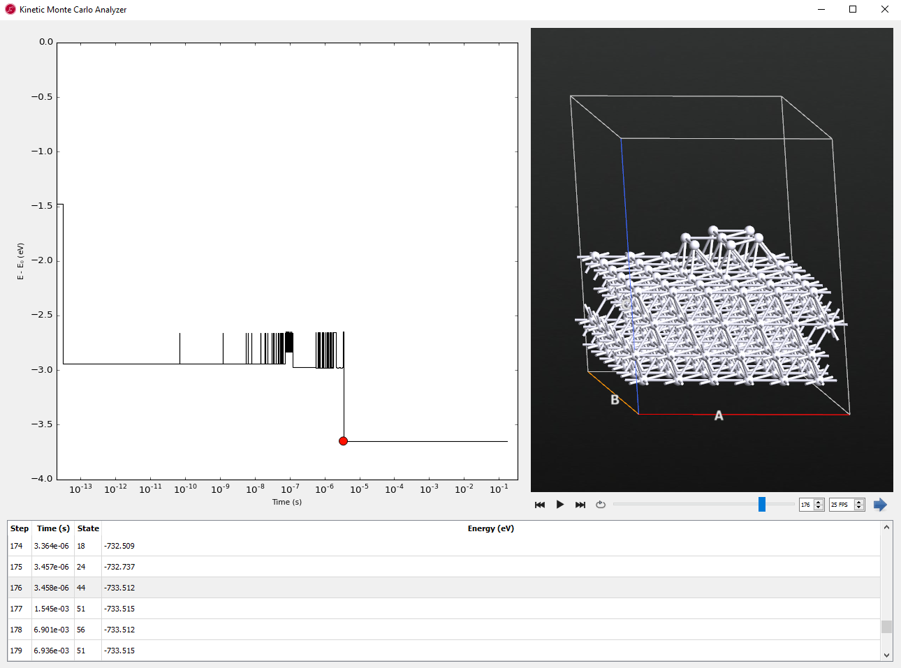
The Kinetic Monte Carlo Analyzer shows a plot of energy vs. time during the AKMC simulation on the left and the geometry of the currently selected configuration/time step on the right.
Tip
You can click on the image to see a version with higher resolution.
The above image shows the results after 1000 saddle searches, which results in the simulation of about 0.17 s of dynamics. The compact island was formed at KMC step 176, which corresponded to a simulation time of 3.4 ms. After the compact island is formed, the entire island diffuses across the surface using a concerted sliding mechanism.
When you click the play  button, you see the dynamics along time.
Markov Chain Analyzer
The Markov Chain Analyzer allows you to look at which reactions are present at each step of the KMC simulation. It can be invoked in two ways:
From the Kinetic Monte Carlo Analyzer by double clicking on a entry in the table.
By selecting the object
in the akmc_markov_chain.hdf5on the LabFloor and clicking the Markov Chain Analyzer… button in the panel.
If we go to the first line in the table in the Kinetic Monte Carlo Analyzer and double click the line, it will open the Markov Chain Analyzer for the initial state.
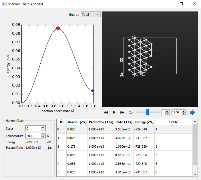
Each of these reaction mechanisms has a very small barrier, indicating that the initial configuration is very unstable. By selecting different mechanisms from the table, each can be visualized. Now we will examine what reaction mechanisms are present for the compact island. Double-click on the line with the 176th step, which is where we found the island formation in the Kinetic Monte Carlo Analyzer. This will take us to state 44, which is the first state containing the compact island.
Note
Remember that the step number is most likely different in your simulation because of its randomly selected initial structure and dynamics.
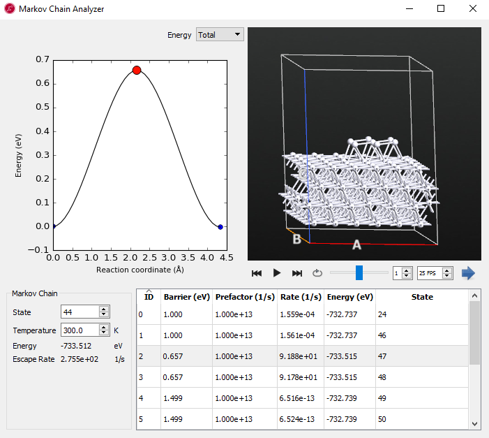
The compact island shows several reaction mechanisms. Each corresponds to the entire 7 atom island diffusion in concert. The barriers are much larger (> 0.65 eV) than those from the initial state and explain why once the compact island is formed a large amount of time passed during the KMC simulation.
The increase in reaction barriers from the initial state with disconnected adatoms to the final compact island shows that the diffusion coefficient of the adatoms decreases dramatically over the course of the simulation.
Conclusion
In this tutorial, we looked at how to model surface diffusion of Pt adatoms using a simple Morse interaction potential. The initial configuration was 7 lone Pt adatoms and the final configuration was a compact 7 atom island. The AKMC simulation modeled longer than 0.1 s of dynamics and the formation time of the compact island took 3.4 ms at 300 K. If a molecular dynamics simulation with a 1 fs timestep had been performed instead, it would have taken 3.4 billion steps to reach the compact island formation. Thus the use of AKMC allowed us to model reaction dynamics on a timescale that is virtually unaccessible using molecular dynamics.