MRAM workflow in QuantumATK: Study of STT-MRAM free layer stability

Version: U-2022.12

Downloads & Links

MRAM builder
Basic QuantumATK Tutorial
ATK Reference Manual
Vampire

This video tutorial will introduce the QuantumATK interface to the Vampire code and use it to calculate the free layer stability factor in a STT-MRAM magnetic tunnel junction structure. The stability factor is obtained from atomistic spin dynamics simulations using Vampire with input parameters obtained from density functional theory (DFT).

Video

Introduction

Spin transfer torque magnetic random access memory (STT-MRAM) is currently being used as standalone and embedded MRAM in modern technology nodes. Further enhancement of the application of STT-MRAM as last level cache requires optimization of the performance and scalability of the magnetic tunnel junction (MTJ) stacks comprising the reference and free magnetic layers as well as additional tunnel barrier and capping layers. The main parameters to optimize in a STT-MRAM are

• Reading. This is determined by the tunneling magneto resistance (TMR), which can be calculated using DFT-NEGF in QuantumATK.

• Writing. The writing operation depends on multiple parameters such as spin transfer torque, magnetic moment of the free layer, and Gilbert damping. These quantities can also be studied with QuantumATK.

• Storage. The storage is characterized by the stability factor \(\Delta = \frac{\Delta E}{k_B T}\), where \(\Delta E\) is the anisotropy energy at the operating temperature \(T\). This is the topic for this tutorial.

Engineering the MTJ to co-optimize the three main requirements of reading, writing, and storage is an active area of research and development.

In this video tutorial we demonstrate a work-flow for calculating the stability factor based on atomistic calculations. Below we summarize the main steps in the work flow, but leave the details to the video.

Workflow for calculating the free layer stability in a STT-MRAM MTJ structure

In the tutorial we adopt the following workflow

• Setup the structure using the MRAM Builder and perform structural relaxation with machine-learned forcefield of the moment tensor potential (MTP) type.

• Calculate Heisenberg exchange coupling parameters and uniaxial anisotropy energies with the HeisenbergExchange and MagneticAnisotropyEnergy objects using DFT.

• Setup and run Vampire simulations using the Vampire Scripter and analyze the results.

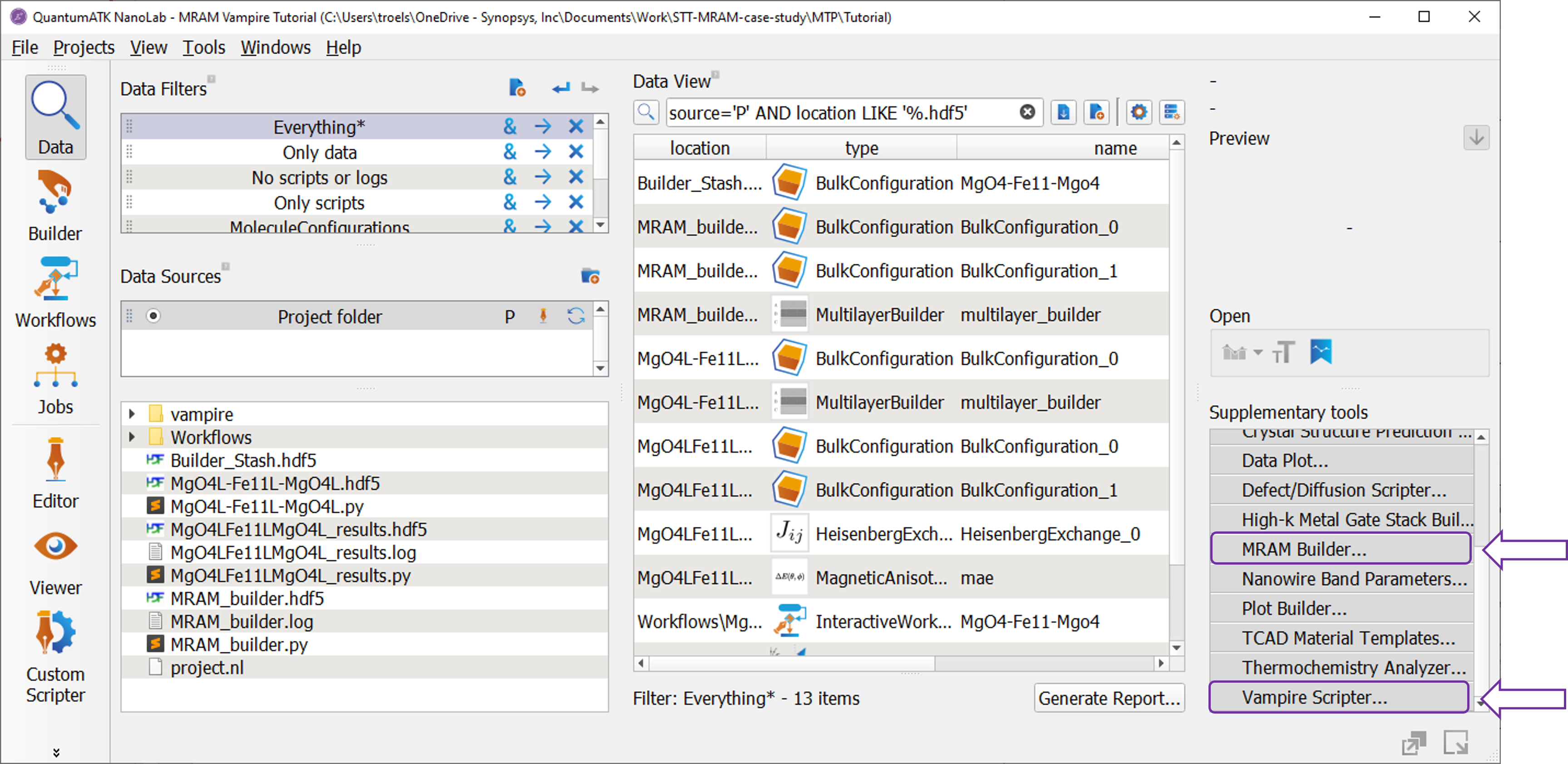
The figure below shows where to find the MRAM builder used for building the MTJ structure, and the Vampire Scripter used for setting up the Vampire simulations.

Vampire

The Vampire simulation tool enables you to perform a range of different atomistic spin dynamics simulations. Common to them all is the basic description of the spin Hamiltonian of the system. While parameterizations of the spin Hamiltonian exist for bulk materials, it is important to note that several of these parameters change significantly in nano-structured systems and in particular at interfaces between different materials. It it thus advantageous to couple DFT calculated parameters with the Vampire simulations.

Spin Hamiltonian

The starting point for atomistic spin dynamics simulations performed in Vampire is the spin Hamiltonian

\[H = -\sum_{i<j}J_{ij} \,\mathbf{S}_i \cdot \mathbf{S}_j - \sum_i k_{i} (\mathbf{S}_i\cdot \mathbf{e}_z)^2 - \sum_i \mu_i \,\mathbf{B}_{app} \cdot \mathbf{S}_i\]

where \(J_{ij}\) are the Heisenberg exchange coupling parameters that can be calculated in QuantumATK using the HeisenbergExchange analysis object. The spin vector \(\mathbf{S}_i\) is a normalized vector with the local spin moment direction on atom \(i\), and \(k_{i}\) is the uniaxial anisotropy energy for atom \(i\), which can be calculated in QuantumATK using the MagneticAnisotropyEnergy study object, and \(\mathbf{e}_z\) is a unit vector along the z-direction. \(B_{app}\) is an externally applied field and \(\mu_i\) is the local spin moment of atom \(i\).

More information can be found on the Vampire home page and in refs. [1] and [2]. Please cite these papers appropriately if using Vampire in scientific publications.

Vampire scripter

When opening the Vampire Scripter, you need to drag-and-drop a HeisenbergExchange onto the first tab in the scripter. This is always required. For magnetic anisotropy energy calculation, you should also provide a MagneticAnisotropyEnergy object since this is responsible for the uniaxial anisotropy constant giving rise to to the anisotropy energy. The first tab is also where you specify the configuration size and shape as well as the simulation cell.

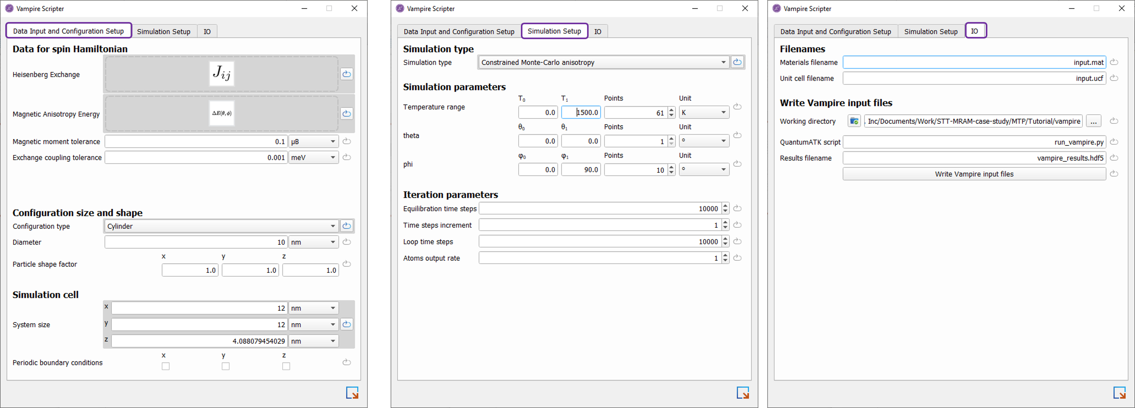
In the second tab you specify the simulation type and various parameters, while in the third tab you specify filenames and where to run the simulation.

Anisotropy energy

Using the constrained monte-carlo (CMC) anisotropy method in Vampire [2], it is possible to calculate the anisotropy energy \(\Delta E(T)\), as shown in the tutorial. This differs from the uniaxial anisotropy energy, \(\Delta E_0\), obtained from the MagneticAnisotropyEnergy study object by being evaluated at a finite temperature, whereas \(\Delta E_0\) is a zero-temperature result. Also, the \(\Delta E(T)\) obtained from the Vampire simulation is obtained from the large cylindrical structure, whereas the \(\Delta E_0\) from the MagneticAnisotropyEnergy study object is obtained from the unit cell. There is thus an area factor difference such that at 0 K we thus expect \(\Delta E(0K) / \Delta E_0 \approx \pi R^2/A_{uc}\), where \(A_{uc}\) is the unit cell area.

The figure shows two of the analysis tabs in the the Magnetic Anisotropy Analyzer used for visualizing and analyzing the result of the Vampire CMC anisotropy simulation. From the MAE value at 300 K \(\Delta E(300K)=0.729\,{\rm eV}\) we manually obtain the magnetic stability factor for the 10 nm diameter cylinder

\[\Delta_{10 nm} = \frac{\Delta E(T)}{k_B T} = \frac{0.729 eV}{0.0258} = 28\]

For 10 years of retention, one typically requires \(\Delta=60\). Assuming that \(\Delta E\) is proportional to the area, this would require a cylinder with a diameter of

\[\frac{\Delta=60}{\Delta_{10 nm}} = \frac{\pi D}{\pi (10\,{\rm nm})^2} \Rightarrow D = 10\,{\rm nm} \sqrt{\frac{60}{28}}\approx 15\,{\rm nm}\]

References

[1]

R F L Evans, W J Fan, P Chureemart, T A Ostler, M O A Ellis, and R W Chantrell. Atomistic spin model simulations of magnetic nanomaterials. Journal of Physics: Condensed Matter, 26(10):103202, feb 2014. URL: https://dx.doi.org/10.1088/0953-8984/26/10/103202, doi:10.1088/0953-8984/26/10/103202.

[2] (1,2)

P. Asselin, R. F. L. Evans, J. Barker, R. W. Chantrell, R. Yanes, O. Chubykalo-Fesenko, D. Hinzke, and U. Nowak. Constrained Monte Carlo method and calculation of the temperature dependence of magnetic anisotropy. Phys. Rev. B, 82:054415, Aug 2010. URL: https://link.aps.org/doi/10.1103/PhysRevB.82.054415, doi:10.1103/PhysRevB.82.054415.