Simulating Thin Film Growth via Vapor Deposition

Introduction

In this tutorial you will learn how to use QuantumATK to run molecular dynamics (MD) simulations to simulate thin film growth onto a substrate via vapor deposition processes.

Vapor deposition is a widely used technique for the production of thin films composed of crystalline or amorphous solids on a substrate material. Simulations of such processes can help understand the underlying microscopic mechanisms, and the effect of the process parameters such as pressure, temperature, etc. on the resulting atomistic structure and kinetics.

In this tutorial you will simulate the growth of silicon carbide (SiC) onto a crystalline SiC substrate, similar to the study in Ref. [1]. You will use empirical potentials which facilitate the simulation of larger systems and time scales than accessible in ab-initio methods, such as DFT. The simulations shown in this tutorial primarily fall under the category physical vapor deposition (PVD). However, chemical vapor deposition (CVD) processes can, in principle, be simulated as well, given that either suitable force fields to describe the chemical reactions are involved, or sufficient computational resources for the use of ab-initio methods are available.

For this tutorial you should be familiar with the basic functionalities of molecular dynamics as described in the How to Setup Basic Molecular Dynamics Simulations. You will learn how to use Python scripting together with the hook functionality available in QuantumATK’s molecular dynamics routines to run advanced simulations.

Note

The exact modified embedded atom model (MEAM) potential used in Ref. [1] is currently not available in QuantumATK. Instead, you will use a Tersoff potential, which, unfortunately, will not produce the crystalline layers shown in the reference paper. The simulation technique, though, is of course independent of the exact potential, and can be used for all kinds of materials.

Note

The limited accessible simulation time requires to operate at vapor pressure values, which are considerably higher than in experiments. You should always keep this in mind when you interpret the simulation results. A more detailed discussion can be found in the general remarks section.

Simulation Strategies

There are different techniques to run a deposition simulation. The main difference to conventional equilibrium MD simulations is that the number of particles in the system increases due to the introduction of vapor atoms or molecules. In QuantumATK two strategies are possible in order to achieve this:

1. Run a new simulation for each newly introduced atom or molecule. The entire deposition simulation can then be performed in an outer loop over the deposited atoms/molecules.

2. Keep all atoms or molecules that should be deposited in a reservoir in the simulation cell. For each new deposition event, take one of these atoms out of the reservoir and place it above the substrate.

The first approach has the advantage that only the atoms that are really needed are present in the simulation cell, which improves the efficiency of the simulation. However, in QuantumATK it is not possible to save the entire simulation into a single MDTrajectory object for later visualization and analysis, due to the varying number of atoms. Therefore, the second approach is chosen in this tutorial. When preparing the simulation one has to pay attention that the atoms in the reservoir do not interact significantly with the active part of the system, in particular with the surface at which the adsorption takes place. In the present case, the reservoir will be represented by a crystal that is attached at the bottom of the substrate.

Preparing the System

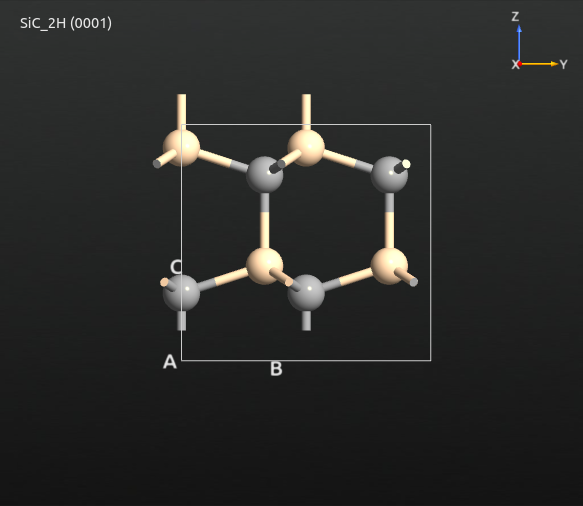
Silicon carbide crystals can occur in different polymorphs. In this tutorial, the substrate will be built from the basic 2H-SiC crystal structure, which is in the configuration database in QuantumATK. You can of course also use a different SiC polymorph to prepare your substrate crystal.

Open the Builder, click Add ‣ From Database, search for SiC, and add the Wurtzite structure.

Preparing the Surface and Reservoir

For this simulation we will consider the (0001) surface of the SiC crystal. To build this surface use the Builders ‣ Surface (Cleave) plugin in the panel bar on the right-hand-side. Select the (0001) Miller indices and a 2x2 surface lattice. Finally, select a Periodic (bulk-like) out-of-plane cell vector and a thickness comprising one layer. Click Finish to finalize the cleaving process.

The resulting cell still has a hexagonal shape in the x-y-plane, which can be inconvenient in MD simulations.

Due to the hexagonal symmetry, the surface lattice can easily be converted into an orthogonal lattice. To this aim open the Bulk Tools ‣ Lattice Parameters widget, select to Keep ‣ Cartesian coordinates, and set the x-component of the B-vector to zero.

Use the Bulk Tools ‣ Wrap plugin to fold the atoms into the new simulation cell, and you will see that the crystal structures remains the same.

Due to the cleaving and wrapping, the termination of the top layer might not always be ideal. In this case, a termination with dangling, i.e. one-fold, coordinated carbon atoms is obtained, which most likely won’t be stable in simulations. To obtain a better termination, shift the entire configuration by invoking Coordinate Tools ‣ Translate, using a z-translation of -0.2 Å, and finally wrapping the configuration into the box via Bulk Tools ‣ Wrap. The final termination should look like the following, featuring a more stable termination at bottom and top.

The next step is to create a supercell of suitable size via Bulk Tools ‣ Repeat. Use a 3x3 repetition in the A-B-plane. The C-vector must be repeated in such a way that a substrate with sufficient crystal layers is created, as well as a reservoir containing enough of atoms to form the desired thickness of the deposited film. For the present example, use 3 layers for the substrate. To keep the simulation time reasonably short you will use only one layer for the reservoir, which gives a total number of 4 repetitions along he C-axis in total. If you later want to perform real production simulations, you may of course increase the number of reservoir layers (and the number of steps in the deposition simulation).

Now you need to mark the different parts of the system via tags. First select the upper two layers of the system to be the thermalized substrate, as shown in the schematic picture of the reservoir approach, and tag them with the name “substrate”. Then select the next lower crystal layer as the fixed bottom layer of the substrate, and assign the tag “bottom”. Finally, select the lowest crystal layer as the reservoir with the tag name “reservoir”.

Optimizing the Lattice Constants

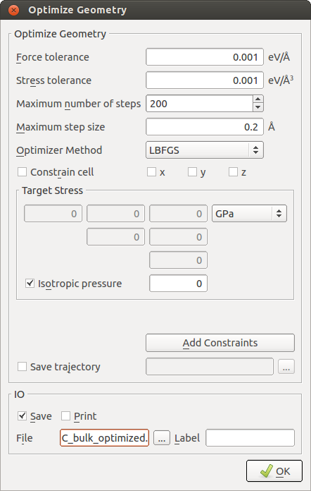
Before building the slab configuration, the bulk system should be optimized under the potential used for the actual deposition simulation to obtain the optimal lateral lattice constants. To this aim send the prepared bulk crystal to the ScriptGenerator, and add a NewCalculator and an Optimize ‣ OptimizeGeometry block. In the New Calculator settings, select ATK- Classical and choose Parameter set ‣ Tersoff_SiC_2005 [2]. Uncheck Print and Save and close the widget. In the OptimizeGeometry settings make the following changes.

Run the simulation and drag the final optimized configuration from the LabFloor to the Builder.

Setting up the Simulation Cell

Finally, a surface has to be created from the bulk crystal. This can easily be achieved by increasing the height of the cell of the optimized bulk system. To this aim, open the Bulk Tools ‣ Lattice Parameters widget. After the optimization, some of the off-diagonal cell components might be slightly different from zero. For convenience they should be reset to zero, while keeping the fractional coordinates constant. To adjust the height of the cell, make sure that you select Keep ‣ Cartesian coordinates. Increase the z-component of the C-vector to 100.0 Å to obtain a sufficient vacuum padding between the active surface and the reservoir.

Setting up the Equilibration Simulation

Before you can run a deposition simulation, the surface has to be thermalized at the desired temperature. In the present example, you will operate at a substrate temperature of 2400 K, as suggested in [1]. Send the prepared configuration from the Builder to the Script Generator. Add a NewCalculator and an Optimize ‣ MolecularDynamics block. In the New Calculator settings, make the same changes as in the previous optimization simulation. In the MolecularDynamics widget, select Molecular Dynamics ‣ Type ‣ NVT Nose Hoover thermostat, 100 000 steps, a log interval of 5000 steps, and enter a suitable trajectory filename. Select Initial Velocity ‣ Type ‣ Maxwell-Boltzmann initial velocities at 2400 K and set the reservoir temperature to 2400 K. (Note that in this case the reservoir temperature does not refer to the particle reservoir in the simulation cell, but denotes the temperature of the virtual heat reservoir, cf. How to Setup Basic Molecular Dynamics Simulations). Uncheck the Save and Print boxes.

Open the constraints widget by clicking the Add constraints button. Both the bottom layer of the substrate and the reservoir atoms should be fixed during the equilibration. This is done by selecting Constraint ‣ Fixed constraints for these two tagged groups and closing the constraints widget.

Run the simulation via the Job Manager or in a terminal using atkpython and use the Movie Tool to send the final snapshot back to the Script Generator.

Setting up the Deposition Simulation

The deposition simulation consists of a normal, long MD simulation, which uses the hook functionality to perform a custom operation after each MD step (cf. MDTrajectory in the reference manual). In this case, at regular intervals an atom is taken from the reservoir and placed above the surface with a random thermal velocity, which is directed towards the active surface. This customized hook function has to be defined in the script using the Python programming language.

To set up the MD simulation in the ScriptGenerator, add a New Calculator and an Optimize ‣ Molecular Dynamics block, and adjust the calculator settings as shown above. In the Molecular Dynamics widget, select the NVT Nose Hoover type, 800 000 steps, a log interval of 2500 steps, and a suitable trajectory filename. Set a reservoir temperature of 2400 K and select Configuration Velocities as initial velocities. Uncheck Save and Print. Send the simulation script to the Editor to make the necessary modifications.

Implementing the Deposition in the Script

At first you have to import the wrap() function to wrap coordinates back into the simulation cell.

from NL.CommonConcepts.Configurations.Utilities import wrap

Then you have to define the class that implements the hook function (the general procedure is similar to the tutorial about Young’s modulus of a CNT with a defect). First, define the class name and its constructor method.

# ------------------------------------------------------------
# Define a hook class to deposit atoms from the reservoir
# onto the active surface of the substrate.
# ------------------------------------------------------------

class VaporDepositionHook:
    def __init__(self,
                 deposition_interval,
                 configuration,
                 substrate_atoms,
                 vapor_temperature=300.0*Kelvin):
        """
        Constructor
        """
        # Store the parameters.

        # The interval after which a new atoms is deposited.
        self._deposition_interval = deposition_interval

        # Store the original coordinates. They will be used to constrain the reservoir atoms.
        self._original_coordinates = configuration.cartesianCoordinates().inUnitsOf(Angstrom)

        # The indices of the atoms that should not be deposited
        self._substrate_atoms = substrate_atoms

        # The vapor temperature.
        self._vapor_temperature = vapor_temperature

        # Deposition count.
        self._deposited_index = 0

        # Get the atoms in the reservoir, i.e. all with z-coordinates lower
        # than the fixed bottom of the substrate.
        self._lowest_substrate = self._original_coordinates[self._substrate_atoms, 2].min()
        self._reservoir_indices = numpy.where(self._original_coordinates[:, 2] < self._lowest_substrate - 0.1)[0].tolist()

        # Get the lattice vectors.
        cell = configuration.bravaisLattice().primitiveVectors().inUnitsOf(Angstrom)
        self._lx = cell[0, 0]
        self._ly = cell[1, 1]
        self._lz = cell[2 ,2]

In the constructor, you essentially store the needed parameters for the deposition, such as the interval at which a new atom is taken from the reservoir, and the original coordinates to constrain the atoms in the reservoir.

Finally, you have to define a method that is called whenever the hook function is invoked. Since our hook is implemented as a Python class, the __call__() method must be defined to make it behave like a function. All hook functions must take the arguments step, time, and configuration. This method should be implemented as follows.

    def __call__(self, step, time, configuration, forces, stress):
        """ Call the hook during MD. """
        # Get the coordinates.
        coordinates = configuration.cartesianCoordinates().inUnitsOf(Angstrom)

        # The reservoir is composed of all atoms that are below the bottom
        # layer of the substrate
        # or above the ceiling of the cell.
        self._reservoir_indices = numpy.where((coordinates[:, 2] < self._lowest_substrate - 0.1) |
                                              (coordinates[:, 2] > self._lz))[0]

        # Freeze the reservoir atoms and reset their positions at every step.
        velocities = configuration.velocities()
        velocities[self._reservoir_indices, :] = 0.0*Angstrom/fs
        configuration._changeAtoms(indices=self._reservoir_indices,
                                   positions=self._original_coordinates[self._reservoir_indices]*Angstrom)

At first, the cartesian coordinates are extracted form the current configuration. Then the atoms in the reservoir are determined based on whether their current position is either underneath the substrate or outside the upper cell boundary. For all reservoir atoms the velocities are set to zero, as we do not want them to move, in particular when the reservoir is increasingly eroded by removing atoms from it. Additionally, their positions are reset to the original positions at the beginning of the deposition simulation.

The next part contains the actual deposition of a new atom from the reservoir, and it is therefore only executed once at the beginning of each deposition interval.

        # Check if it is time for the deposition of a new atom from the reservoir.
        if (step % self._deposition_interval) == 0:
            # Get elements and velocities.
            elements = numpy.array(configuration.elements())
            velocities = configuration.velocities().inUnitsOf(Angstrom/fs)

            # If the reservoir is empty, do nothing.
            if len(self._reservoir_indices) == 0:
                return

            # Decide which element to deposit next.
            possible_elements = [Silicon, Carbon]
            element_index = self._deposited_index % 2
            next_element = possible_elements[element_index]
            reservoir_elements = elements[self._reservoir_indices]

            # Get the element candidates.
            possible_atoms = numpy.where(reservoir_elements == next_element)[0]

            # If not avaiblable, try the other element.
            if len(possible_atoms) == 0:
                next_element = possible_elements[element_index-1]
                possible_atoms = numpy.where(reservoir_elements == next_element)[0]

            # Return back the global atom indices.
            possible_atoms = self._reservoir_indices[possible_atoms]

            # Pick an atom at the bottom of the reservoir
            lowest_atom = numpy.argmin(coordinates[possible_atoms, 2])
            next_index = possible_atoms[lowest_atom]

            # Place the deposition atom above the surface at a random lateral position.
            new_coords = numpy.array([numpy.random.uniform()*self._lx,
                                      numpy.random.uniform()*self._ly,
                                      self._lz - 15.0])

            configuration._changeAtoms(indices=[next_index], positions=new_coords*Angstrom)
            wrap(configuration)

            # Draw random velocities for the atom according to
            # Maxwell-Boltzmann at the specified temperature.
            m = next_element.atomicMass()
            sig = self._vapor_temperature*boltzmann_constant/m
            sig = sig.inUnitsOf(Ang**2/fs**2)
            sig = numpy.sqrt(sig)

            new_velocity = numpy.random.normal(scale=sig, size=3)
            velocity_norm = numpy.linalg.norm(new_velocity)

            # Set the velocity so that it points towards the active surface.
            new_velocity = numpy.array([0.0, 0.0, -velocity_norm])
            velocities[next_index] = new_velocity

            # Set the new velocities on the configuration.
            configuration.setVelocities(velocities*Angstrom/fs)

            self._deposited_index += 1

# ------------------------------------------------------------
# End of hook class definition
# ------------------------------------------------------------

We start by determining which element has to be deposited next. As silicon and carbon are deposited in an alternating manner, this can easily be detected by querying whether the current deposition index is an odd or even number. Then all reservoir atoms of this element are selected and the atom which resides deepest at the bottom of the reservoir is picked. If for some reason no element of the requested type is available in the reservoir, we simply pick the other element instead. New random lateral coordinates, as well as a height at 15.0 Angstrom below the cell ceiling are created and assigned to the deposition atom via the _changeAtoms() method of the configuration. For better visibility, the coordinates are folded back into the cell using the wrap() function. To model the vapor temperature of the deposition atoms, new velocities are drawn from a Maxwell-Boltzmann distribution and, to ensure that the atom travels towards the surface, the velocity vector is re-aligned. For simplicity, the vector always points vertically to the surface, but in general, different impact angles can easily be implemented, as well. The new velocites are assigned to the deposition atom and the configuration velocities are updated using the setVelocities() method. Finally, the running deposition index is incremented, completing the class definition.

After the definition of the VaporDepositionHook class, a new instance is initiated, and the parameters for the current simulation are specified. This should be done immediately before the Molecular Dynamics block in the script.

# Initialize the hook class.
deposition_hook = VaporDepositionHook(deposition_interval=5000,
                                      configuration=bulk_configuration,
                                      substrate_atoms=substrate+bottom,
                                      vapor_temperature=2400.0*Kelvin)

To run the simulation, use the pre-defined MD block from the Script Generator with only two slight modifications. In the method definition of the Nose–Hoover thermostat, the reservoir_temperature parameter is modified, so that only the group of atoms marked by the “substrate” tag is coupled to the thermostat.

# Define an NVT thermostat where only the substrate atoms are thermalized.
method = NVTNoseHoover(
    time_step=1*femtoSecond,
    reservoir_temperature=[('substrate', 2400*Kelvin)],
    thermostat_timescale=100*femtoSecond,
    heating_rate=0*Kelvin/picoSecond,
    chain_length=3,
    initial_velocity=initial_velocity
)

This is necessary, to ensure that the dynamics of the deposited atoms in the gas phase are not spuriously modified by the thermostat before they have adsorbed to the surface (i.e. the deposited atoms should be in the NVE ensemble). Finally, the deposition_hook object must be passed as an argument to the MolecularDynamics() function.

md_trajectory = MolecularDynamics(
    bulk_configuration,
    constraints=bottom,
    trajectory_filename='SiC_deposit_tutorial_md.nc',
    steps=800000,
    post_step_hook=deposition_hook,
    log_interval=2500,
    method=method
)

The complete script for the entire simulation can be found in the file Script_deposit_SiC.py.

Note

In QuantumATK version 2016, the NVT Nose–Hoover method is implemented in the NVTNoseHoover class, which is the one used in the script provided above. However, in QuantumATK version 2015 and earlier, that class is named NVTNoseHooverChain. The script provided above will therefore not work with QuantumATK 2015 and earlier. Use instead this script: Script_deposit_SiC_atk2015.py.

Running the Simulation

Run the script via the Job Manager or in a terminal. Such a long MD simulation might take a couple of hours to complete. You may notice that some atoms, instead of adsorbing to the surface, are scattered back into the vapor phase. This is not a problem, though, as these atoms, while travelling upwards, will eventually reach the reservoir, where they will automatically be treated as normal reservoir atoms again.

The following figure displays snapshots at different stages of the deposition simulation.

At first, only few atoms have been deposited onto the surface and adsorb forming single adatoms. With more and more atoms being deposited a first layer begins to form above the substrate surface. The first layer still resembles, at least partially, the crystalline structure of the substrate, whereas subsequent layers reveal a more amorphous structure. This must be attributed primarily to the employed potential (see the note at the beginning), but to some extent also to the high deposition frequency, as specified by the deposition_interval parameter. A larger value for this parameter will decrease the deposition frequency, which may allow for a more controlled integration of the deposited atoms. Remember, if you increase the deposition interval, you have to increase the total number of steps in the deposition simulation by the same factor to make sure all the atoms in the reservoir are being deposited.

Notice how at the same time as the film grows, the reservoir region at the bottom of the slab is depleted, as more and more atoms are taken away. However, the special constraints in the script make sure that the vanishing structure does not de-stabilize the entire system.

General Remarks

This simulation technique is, in principle, applicable to all kinds of materials. Of course, you might need to make several modifications in the script, such as adapting the elements. Instead of single atoms, you can also deposit entire molecules. For production simulations you may want to increase the number of layers in the reservoir to obtain a larger deposited film. Feel free to play around with other parameters, e.g. temperature, or the deposition interval. The deposition frequency, i.e. the inverse of the deposition interval, can be associated with the vapor pressure via the Hertz–Knudsen equation (cf. for instance [3]):

$$\frac{dN_i}{dt} = \frac{p_i A}{\sqrt{2 \pi m_i k_B T}} \, ,$$

where $p_i$ denotes the partial pressure of element/molecule i, A the surface area, and $m_i$ the atomic/molecular mass.

Inserting the parameters from the simulation, you will find that the corresponding vapor pressure is around 66 bar, which is far away from the typical experimental near-vacuum conditions. This aspect represents a considerable shortcoming of such simulations, as the accessible simulation time in most cases prevents the use of realistic pressure values, rendering a time-resolved interpretation of the growth kinetics very difficult. Essentially, it means that the particles impact at a too high rate, which can, for instance, result in an increased local heating, as the reaction heat cannot be transported sufficiently fast from the surface to the thermostatted bulk substrate. However, the obtained structural model of deposited films can in most cases be considered a good approximation to the real film structure. You should bear in mind the conditions, though, under which the simulation has been performed and reconsider whether these conditions might have an influence on the deposited structure.

Furthermore, note that the use of a constant deposition interval provides another approximation, as the real process might rather follow a Poisson distribution than a uniform distribution. Although a Poisson distribution can easily be implemented into the script (using e.g. python’s random.poisson function), this would primarily make sense if the deposition interval can actually be chosen high enough to reproduce the desired real vapor pressure.

References

[1] (1,2,3)

Kang, K.-H; Eun, T.; Jun, M.-C.; Lee, B.-J.: Governing factors for the formation of 4H or 6H-SiC polytype during SiC crystal growth: An atomistic computational approach. J. Cryst. Growth, 389, 120 (2014)

[2]

P. Erhart and K. Albe: Analytical potential for atomistic simulations of silicon, carbon, and silicon carbide. Physical Review B, 71, 035211, (2005)

[3]

K. Reuter: First-Principles Kinetic Monte Carlo Simulations for Heterogeneous Catalysis: Concepts, Status, and Frontiers. in “Modeling Heterogeneous Catalytic Reactions: From the Molecular Process to the Technical System”, Wiley-VCH (2011)