Advanced device relaxation - manual workflow
In this tutorial you will learn how to use a combination of “Rigid” constraints and a simple optimization routine to perform efficient and reliable relaxation of the internal coordinates in a device configuration.
Note
In the O-2018.6 release, we introduced a so-called Study Object to automate the workflows described in this tutorial. That is now the recommended way of performing device geometry optimizations in QuantumATK, and if you have access to O-2018.06 or newer, you should go to the corresponding tutorial Relaxation of devices using the OptimizeDeviceConfiguration study object. Users of previous versions can still perform the calculations using the more complex workflow, that is described here.

Introduction
Relaxation of the internal coordinates of device configurations can be a tedious and time consuming task. There are two main reasons for this:
The 2-probe configuration consists of three distinct regions: Two electrodes and a central region consisting of electrode extensions and a scattering region. The geometry of each region should be separately optimized in a first-principles manner, but both electrode extensions in the central region must always match the corresponding electrode.
Step 1: Optimize the electrodes. After optimization of the electrodes, it is important to make sure that the electrode extensions in the central region match the optimized electrodes.
Step 2: Optimize the central region. The optimum length of the central region is usually not known a priori. In the case of a periodic bulk, one would minimize the stress tensor. However, the stress field is not uniquely defined for a device configuration, so another approach is needed.
In the second step, we must rely on minimizing the device total energy while explicitly preserving the internal coordinates of the electrode extensions. There are at least two different ways to do this using QuantumATK.
BRR method
After building the 2-probe configuration from fully relaxed electrodes, you extract the central region bulk and relax it with “Rigid” constraints on the atoms belonging to the electrode extensions. The device or interface is then reassembled from the relaxed bulk. This is a computationally efficient approach and will usually capture a large fraction of the required geometry relaxation. We shall refer to this method as Bulk Rigid Relaxation (BRR).
The BBR method does not calculate the total energy using a full device geometry, so the reassembled device may not be exactly in the global minimum-energy geometry. Some types of electronic structure calculations may be sensitive to this difference, others may not.
1D minimization
A somewhat more brute-force approach is to explicitly minimize the device total energy wrt. internal coordinates and the central region length, i.e., do the full 2-probe calculations and vary the central region length. This is a 1D minimization problem with relaxation of the atomic positions at each step, so we shall refer to this method as 1DMIN. We have developed a procedure for doing this as efficiently as possible with QuantumATK, but the computations are in general more demanding than with BRR. It is therefore recommended to use 1DMIN only after pre-relaxing the central region with the BRR method.
This tutorial introduces the electrode relaxation and the central region relaxation using BRR and 1DMIN methods. The methods are illustrated for relaxing a silver-gold interface using a classical potential. The classical potential is selected for computational convenience, and the same procedure could be used for another relaxation method like DFT. In general we recommend to check ATK-ForceField calculations with DFT calculations.
Preparations
First make a new project called ‘device_relaxation’. Our starting
point is an unrelaxed 2-probe device configuration. It was created
using the QuantumATK Interface Builder follow the tutorial at this link:
Building an interface between Ag(100) and Au(111). The geometry can also be downloaded as this file:
Ag_Au_interface.py.
Save the py-file in your project folder, locate the device configuration on the
LabFloor, and drag-and-drop the configuration to the  Builder.
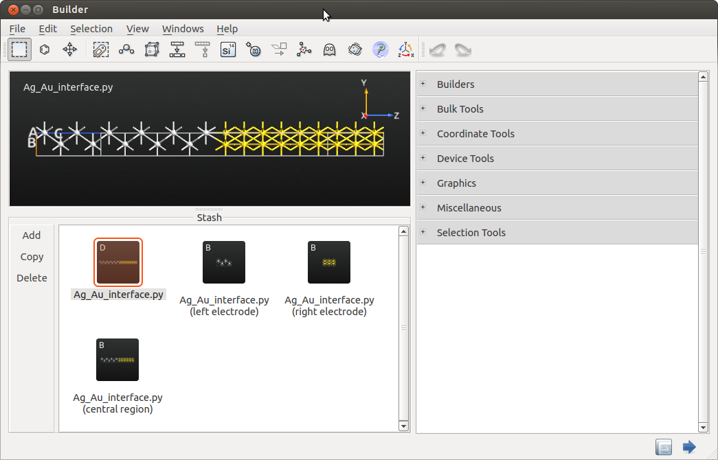
The 2-probe configuration should look like the one illustrated
below. It consists of a left electrode, Ag(100), the central region,
and a right electrode Au(111). Use the  plugin to split
the device into a left electrode, right electrode and central region.
plugin to split
the device into a left electrode, right electrode and central region.
Electrode relaxation
The device geometry was constructed using the interface builder (Building an interface between Ag(100) and Au(111)). Prior to building the interface the left and right crystal structures were set up using their experimental geometries. We will assume that the experimental geometry is also the lowest energy structure of the theoretical method we will use for relaxing the device geometry.
In the interface builder we choose “Strain second surface” upon selecting the surface cell. This means that the Ag(100) surface was kept in its experimental geometry, while the Au(111) surface was strained in the x,y directions upon forming the interface. When the crystal is strained in the x,y directions, it will relax in the z-direction according to the Poisson ratio of the material.
In the following we will apply this relaxation to the Au(111) crystal, by relaxing the stress in the z-direction while keeping the x, y directions fixed. The obtained relaxation of Au(111) will be transferred to the gold atoms in the central region.
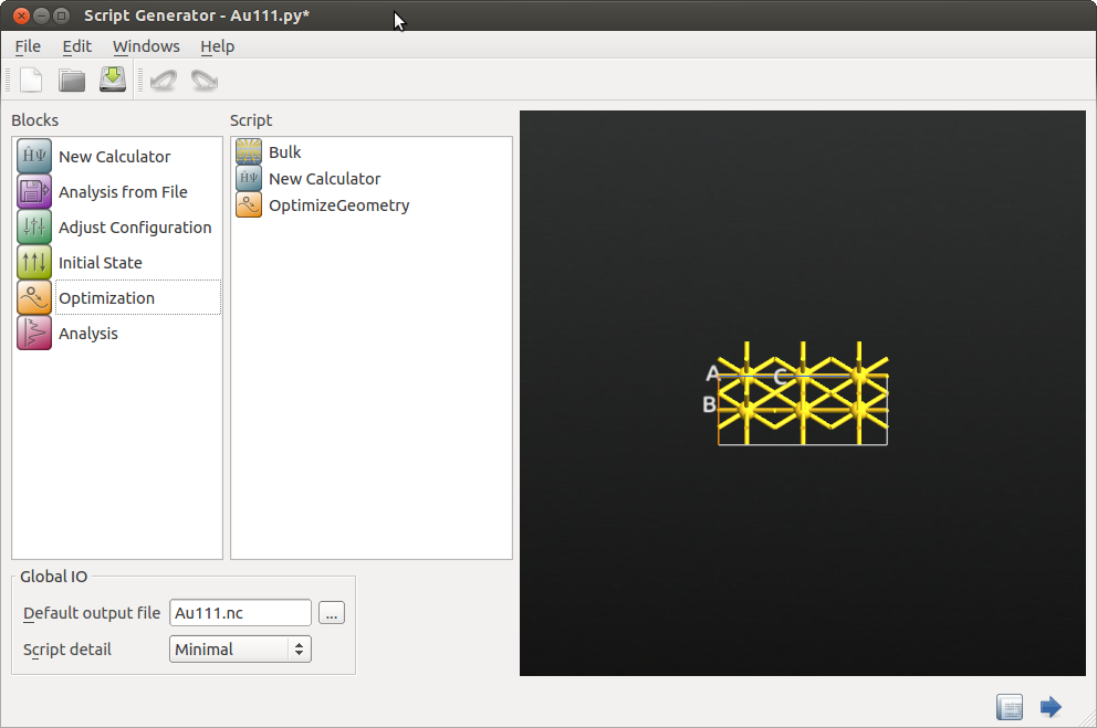
Open the builder and change the name of the right electrode to
Au111. Double click the geometry to make it active and send it to the
 Scripter.
Add the following objects:
Scripter.
Add the following objects:
 New Calculator
 OptimizeGeometry
Now open the New Calculator object and select the ATK-ForceField “EAM_Zhou_2004” potential. Click OK.
Note
For QuantumATK-versions older than 2017, the ATK-ForceField calculator can be found under the name ATK-Classical.
Next open the Optimize Geometry object:
Set the force tolerance to 0.01
Set the stress tolerance to 0.001
Uncheck z in the “Constrain cell” checkboxes

Send the script to the  Job Manager and run the relaxation.
It should take less than a minute to execute. When finished inspect
the log file.
Job Manager and run the relaxation.
It should take less than a minute to execute. When finished inspect
the log file.
You should now see a new object on the LabFloor called “Au111.hdf5”. It
contains two configurations, corresponding to the geometry before and
after the relaxation. Select the two geometries and drop them onto the
 Viewer. In the viewer you can hoover the mouse over the
unit cell of each configuration and you will notice that the length of
the C vector is 7.064 Å before the relaxation and 7.011 after the
relaxation. This information could also be obtained from the log file,
“Au111.log”.
Viewer. In the viewer you can hoover the mouse over the
unit cell of each configuration and you will notice that the length of
the C vector is 7.064 Å before the relaxation and 7.011 after the
relaxation. This information could also be obtained from the log file,
“Au111.log”.
The relaxation results in a small compressive strain of 0.75%. To apply this to the central region, open the Builder and double click the central region configuration.
Rename the stash item to “central”.
Select all the gold atoms by drawing a rectangle around them.
Open the plugin.
Enter 0.9925 along the C axis.
Use “Selected atoms are” stretched.
Click Apply.

Note
The strain is so tiny that it is not possible to see any
visual change in the structure. However, you may open the
“Lattice Parameters..” plugin and click the  and
and  buttons to see how the C cell vector
changes when you undo and redo the stretch.
Similarly, you can inspect the Coordinate List.
buttons to see how the C cell vector
changes when you undo and redo the stretch.
Similarly, you can inspect the Coordinate List.
Central region relaxation
You are now going to relax the central region only. We want the electrode extensions to be able to move freely (but rigidly) during geometry relaxation. We therefore add vacuum on both ends:
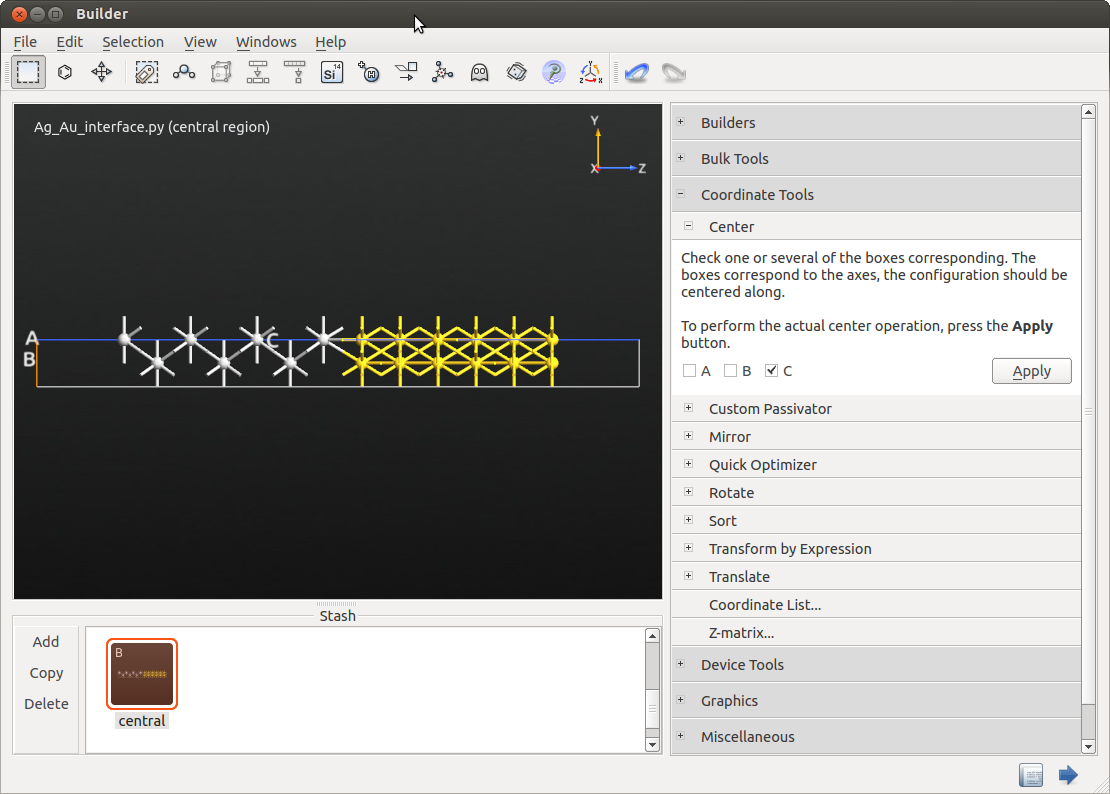
Make sure that no atoms are selected, by clicking the background of the plotting window. In use the C-vector slider to increase the cell length by 30% or simply type in a multiplication factor of 1.3. The cell is stretched once you click Apply.
Move to and uncheck A and B. Center the central region by clicking Apply.
We want to fix the atoms in the electrode extensions by including an additional layer of the central region. The additional layer will help the Device from Bulk tool in QuantumATK to identify the length of the electrode. For this purpose select the 5 outermost silver atoms. Open . Enter Left in the box named “Click here to write a new tag…”. Press Return.
Next select the 4 outermost gold atoms, and tag them Right.

Send the configuration to the Script Generator
and set up the calculation:
Add a New Calculator and an
OptimizeGeometry object.
Choose the ATK-ForceField engine and the “EAM_Zhou_2004” potential for these calculations.
Make the following changes to the OptimizeGeometry object:
Set the force tolerance to 0.01 eV/Å.
Check “Save trajectory” and set the filename to
central.hdf5.Click “Add Constraints” to set up the Rigid constraints on the electrode extensions.
Check that the Left and Right tags are assigned to the correct atoms in the configuration. Do this by clicking the tags. Choose “Rigid” constraints for both tags.
Click OK and return to the Scripter.

Note
Choosing instead a “Fixed” constraint for one of the tagged regions while keeping the other one “Rigid”, may save BFGS relaxation steps and thereby computational time.
Send the script to the Job Manager and run the calculation.
It should be very fast. Once finished, the central.hdf5 output file
appears on the LabFloor.
You can use the Viewer plugin to see the trajectory
of the relaxation as illustrated in the animation below.

The relaxed central region is saved in central.hdf5 as the bulk
configuration with id “glD002”. This is your initial guess for the central
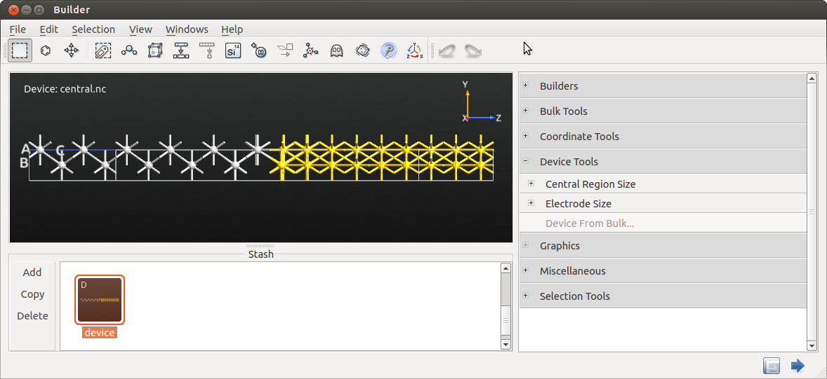
region geometry. Drag-and-dro it on to the Builder.
Click to turn the
central.hdf5 bulk into a device configuration. You can leave the
settings for electrode and central region lengths at default values.
The interface configuration should now look like illustrated below. Rename the configuration to “device” by using F2 or with a right mouse-click.
1DMIN optimization of the interface using 2-probe calculations
We are now ready to search for the global minimum-energy geometry of
the Ag(100)-Au(111) interface. Save the device configuration as a HDF5
file named device_in.hdf5 by choosing “Save as” after
right-clicking the device Stash item.

You are now going to apply a simple SciPy minimization procedure
in search for the central region length that minimizes the interface
total energy. The device configuration you just saved in device_in.hdf5
is the starting point for this.
Two scripts are needed. You can download them here:
device.py and optimize.py. Save both scripts
in the folder where device_in.hdf5 was saved. The first script
(device.py) reads in the device configuration and sets up
and runs the calculation, while the second script
(optimize.py) contains functions and classes used by device.py.
Note
To use the script device.py for other systems you need to edit the script and change the definition of the potential to an appropriate potential for your new system.
Both scripts should now be available in the QuantumATK “Project Files” list.
Drag-and-drop device.py onto Jobs. The Job Manager
will open. Click  to run the script.
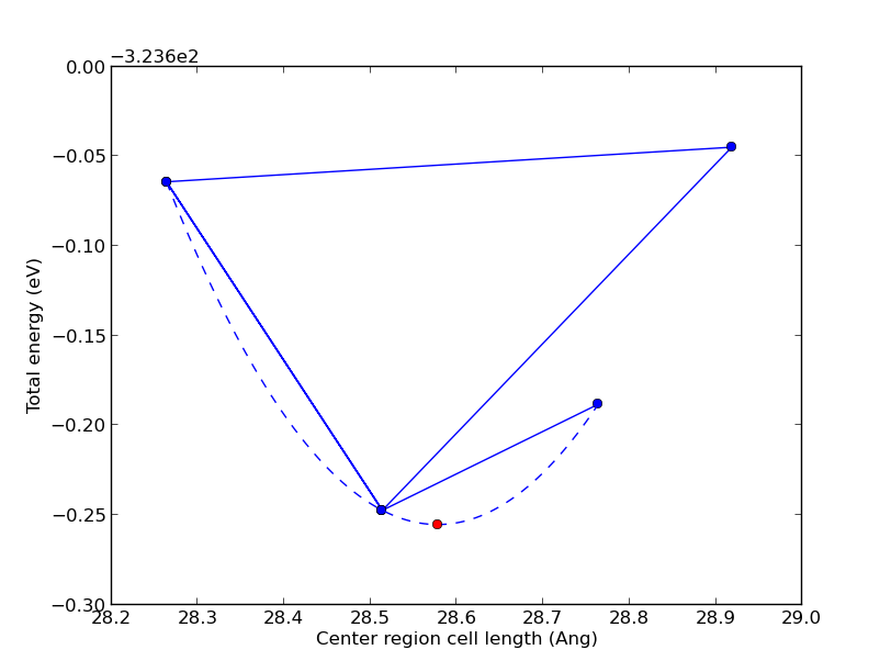
Once finished (it’s fast!), a window with the figure below will pop up. The blue points are total energies of relaxed interface configurations. The initial cell length is 28.51 Å and the other blue points are trial guesses made by the algorithm. The red point indicates the optimum central region length which is 28.58 Å. The optimization routine simply maps out the illustrated potential-energy surface and finds its minimum!
The job will finish when you close the pop-up window.
The relaxed configurations are saved in the output file device_out.hdf5
along with the total energies. The configuration corresponding to the
red point (the final device or interface geometry) is the latest device
configuration (the one with largest id number).
Using the Viewer plugin, the minimum-energy interface
configuration looks like this:

In this case the change to the structure after the 1DMIN relaxation is minute compared to the BRR relaxation. Often the BRR will be sufficiently accurate and there is no need for the 1DMIN step. The 1DMIN approach is only needed for extreme accuracy.