Band Structure, Projected Density of States and Effective Mass Calculations
Band Structure, Projected Density of States and Effective Mass Calculations
Version: Y-2026.03
In this tutorial, you will learn how to use the QuantumATK NanoLab GUI to
Set-up band structure, projected density of states (PDOS) and effective mass calculations for bulk Si and SiO2 (quartz) using Density Functional Theory (DFT).
Analyze obtained results.
All the workflow, input and output files can be found in the Example Project - Y-2026.03 ‣ SiO2-quartz-bandstructure-pdos and Si-bandstructure-effective-masses folders.
To create a workflow for Bandstructure and ProjectedDensityOfStates calculations in the Workflow Builder, follow the step-by-step protocol described below. Here, you will use DFT with LCAOCalculator basis sets. For the DFT functionals, choose a hybrid HSE06 DFT functional for bulk Si (exact exchange fraction of 0.25 optimized for Si) and a dielectric dependent hybrid HSE06-DDH functional (DDHCustomExchangeCorrelation) for SiO2 (quartz) to find an improved material specific exact exchange fraction for more accurate band structure and band gap.
Follow the Geometry Optimization tutorial to optimize the structure of bulk Si and SiO2 (quartz).
In the Builder, click on the Send content to other tools button to send the optimized structures from the Builder Stash to the Workflow Builder.
Go to the Block Catalog ‣ QuantumATK tab ‣ Calculators and Analysis categories on the right hand panel and drag-and-drop the SetLCAOCalculator and Bandstructure blocks, respectively, to the middle Workflow Area ‣ Build tab.
For SiO2 (quartz) case, add a LocalExactExchangeFraction block from the Block Catalog ‣ QuantumATK tab ‣ Analysis category. It will return the calculated improved material specific exact exchange fraction for SiO2 (quartz).
Double-click on the SetLCAOCalculator block and make the following changes:
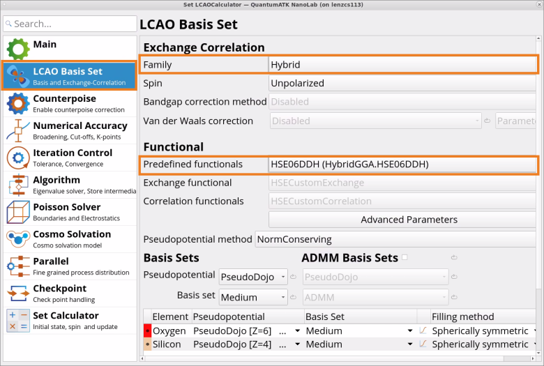
In the LCAO Basis Set tab of the SetLCAOCalculator block, change the Exchange CorrelationFamily from the default GGA to Hybrid with predefined HSEO6 (HybridGGA.HSE06) functional for Si and HSE06DDH (Hybrid.GGA.HSEO6DDH) for SiO2 (quartz).
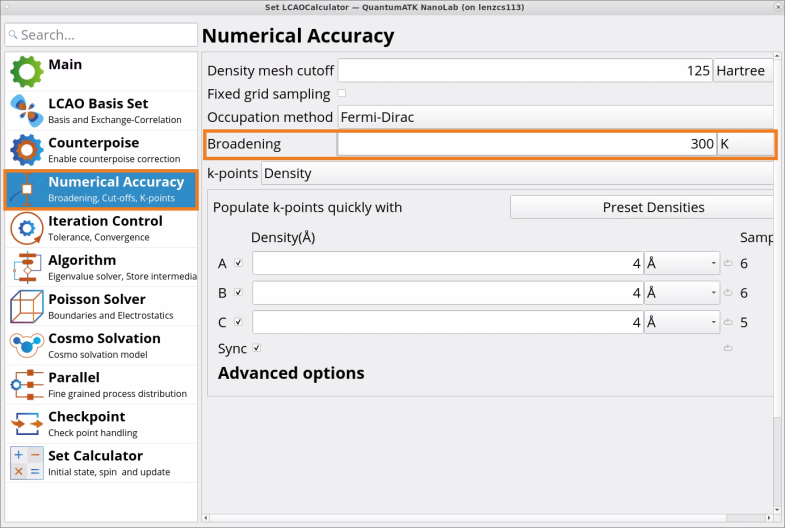
In the Numerical Accuracy tab of the SetLCAOCalculator block, change the numerical accuracy paremeter Broadening from 1000 K to 300 K (recommended for semiconductor materials).
Tip
SetLCAOCalculator block sets medium k-point sampling, medium basis set and 125 Ha density mesh cutoff (system-dependent) by default, typically providing good accuracy results with modest computational resources. It is recommended though to check the convergence of your results with these parameters.
SetLCAOCalculator block uses a default Fermi-Dirac Occupation Method with 1000 K Broadening, which generally works reasonably well across various systems. Another setting may be more appropriate for your system, and you can adjust these settings according to the recommendations in Occupation Methods for semiconductor, insulator, metal, and molecule systems.
For slabs, surfaces and interfaces (modelled as slabs), it is recommended to set FFT2D Poisson Solver (Dirichlet/Neumann) in the out-of-plane (C) direction instead of the default FFT (Periodic) in the SetLCAOCalculator block, Poisson Solver section. For neutral molecules, stick to the default FFT Poisson solver, whereas for charged molecules, set the Multigrid/Multipole Poisson Solver. Read these technical notes on Poisson solvers to learn more.
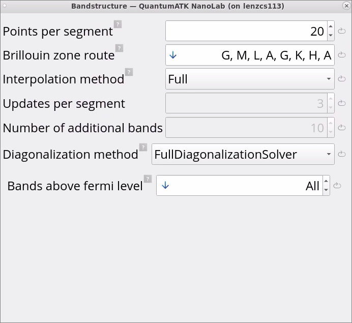
Double-click on the Bandstructure block. Here, the Brillouin zone route is automatically detected, and there is an option to modify it. There is also a possibility to increase the number of points per segment for more fine sampling of bandstructure. Stick to the default settings.
Tip
When calculating band structure of very large systems (> 1000 atoms), there is an option to choose IterativeDiagonalizationSolver instead of FullDiagonalizationSolver in the Bandstructure block to speed-up simulations, in particular with Semi-Empirical Thigh-Binding models for more than order of magnitude faster calculations.
Perform LocalBandstructure calculations to get insights into the local properties of the band structure such as effective masses and band unparabolicity for specified k-point, bands and directions.
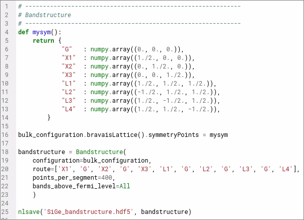
When setting up bandtructure calculations for low symmetry crystal or systems with atomic disorder (e.g., alloys), one needs to define k-routes in the Brillouin zone in a script input.py. For example, for SiGe alloy specify inequivalent X and L points, resulting in degeneracy lifting, i.e., alloy broadening of bands.
Change the Workflow name in the Workflow Stash and Filename as needed (e.g., SiO2-quartz-bandstructure-HSE06-DDH.hdf5).
Click on the Send content to other tools button and choose Jobs as a script to send the workflow to the Jobs tool in order to submit this job on a local machine or a remote cluster. It is recommended to parallelize over both MPI processes and threads in DFT simulations. Read the technical notes on Parallelization of QuantumATK calculations to learn more.
This also generates a Python script SiO2-quartz-bandstructure-HSE06-DDH.py, based on this workflow. It can be opened and edited with the Editor tool and then sent to the Jobs tool.
Once the calculation has finished, we are ready to analyze the results.
Go to the Data View tool.
In the Data Sources select the file SiO2-quartz-bandstructure-HSE06-DDH.hdf5 and then in the Data View window double-click on the Bandstructure_0 object to open it with the Bandstructure Analyzer.
Examine Direct band gap, Indirect band gap, Valence band edge and Conducion band edge reported in the Bandstructure Analyzer.
Zoom into the band structure using Zoom and Plot editor tools and use measuring tools (right-click to Add measurement) to measure direct and indirect bandgaps yourself.
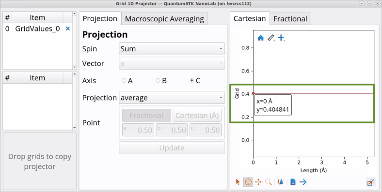
Double-click on GridValues_0 object in Data View to open it with the Grid 1D Projection Analyzer. Examine the automatically calculated exact exchange parameter in HSE06-DDH, which is 0.4 for SiO2 (quartz) - quite different from the pre-set 0.25 exact exchange parameter in the HSE06 functional.
Note
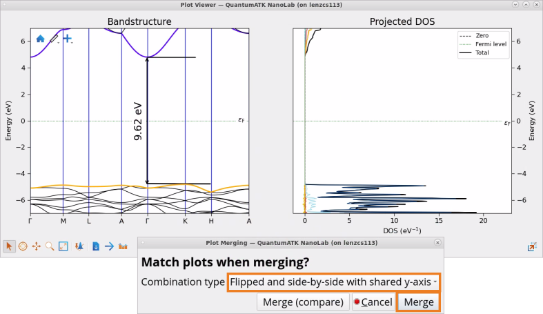
Calculated indirect band gap of SiO2 (quartz) 9.62 eV with the HSE06-DDH functional is in a good agreement with experimental (9.65 eV) [1] and many-body GW method (9.68 eV) [2] results. Indirect band gap obtained with HSE06 is 8.39 eV.
When simulating interfaces between different materials, choose HSE06LocalDDH for the predefined functional in the SetLCAOCalculator block, which automatically calculates material specific exact exchange fractions for each material in the interface.
In QuantumATK it is easy to restart from a previous simulation and calculate additional properties, for example, projected density of states, without re-doing the SCF convergence part. Follow this step-by-step protocol to set up additional projected density of state calculations.
Go back to the Workflow Builder and click on the the Add button to add a new workflow.
Change the Workflow name and Filename as needed (e.g., SiO2-quartz-PDOS-HSE06-DDH.hdf5).
Go to the Block Catalog ‣ QuantumATK tab ‣ Algorithm and Analysis categories on the right hand panel and drag-and-drop the Load from file and ProjectedDensityOfStates blocks, respectively, to the middle Workflow Area ‣ Build tab.
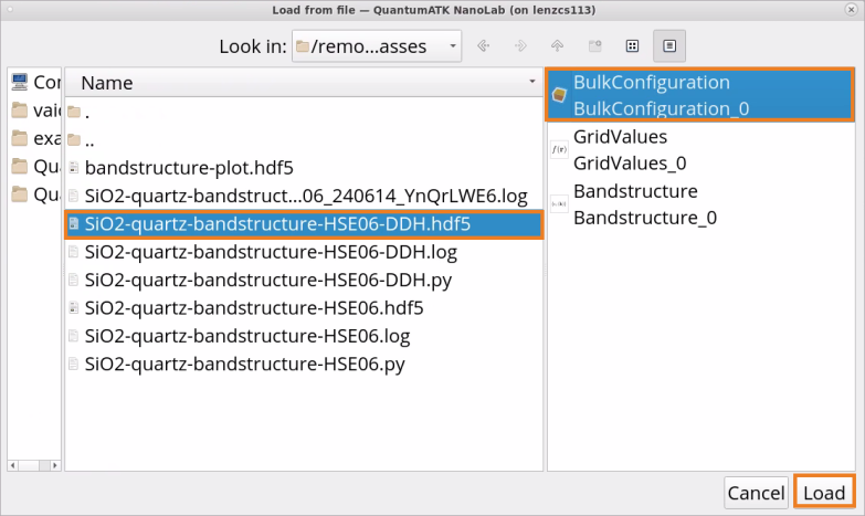
Double-click on the Load from file block to choose from which file to restart the calculation:
Click on Load from file.
Choose to restart from file SiO2-quartz-bandstructure-HSE06-DDH.hdf5 ‣ BulkConfiguration.
Click Load.
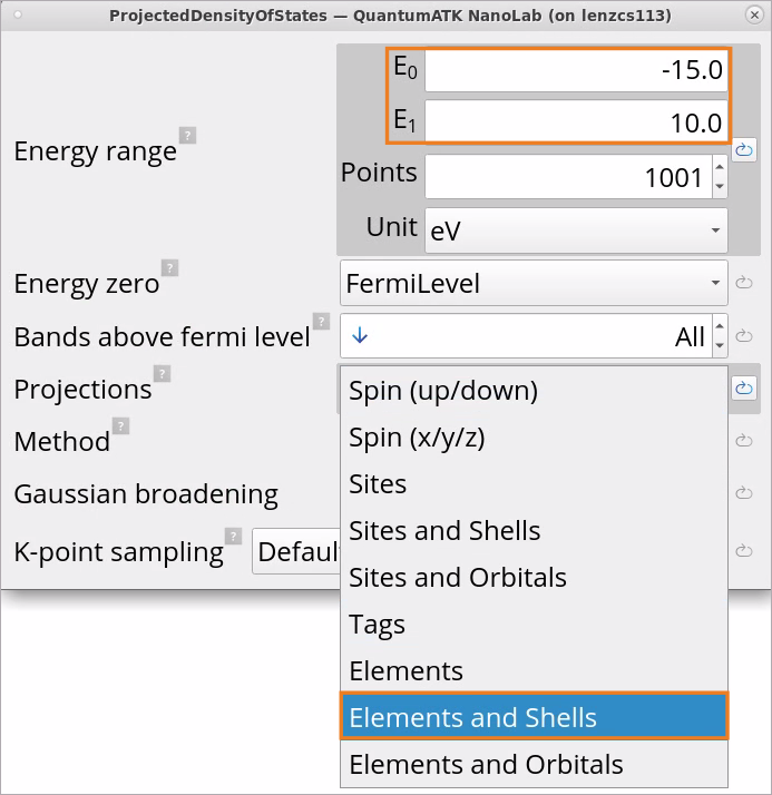
Double-click on the ProjectedDensityOfSates block and make the following edits:
Define an Energy range: default -5 eV ÷ +5 eV is good for Si, but it should be increased for SiO2 (quartz) to -15 eV ÷ +10 eV as it has a much larger band gap than Si.
Choose Projections on Elements and Shells from various options, such as Spin, Sites, Sites and Shells, Sites and Orbitals, Elements, Elements and Shells, Elements and Orbitals.
Select TetrahedronMethod for calculating the projected density of states.
Tip
Choose Projections on Sites to get local density of states / band diagram across interfaces, stacks or inhomogeneous systems in general.
Click on the Send content to other tools button and choose Jobs as a script to send the workflow to the Jobs tool in order to submit this job on a local machine or a remote cluster.
Once the calculation has finished, we are ready to analyze the results.
Go to the Data View tool.
In the Data Sources, select the file SiO2-quartz-PDOS-HSE06-DDH.hdf5 and then double-click on the ProjectedDensityOfStates_0 object in the Data View window to open it with the Projected DOS Analyzer.
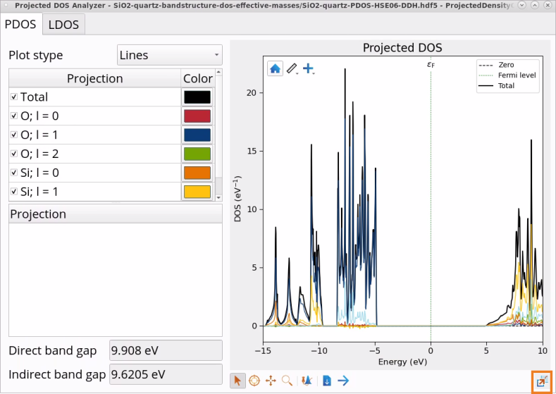
Use Projected DOS Analyzer to visualize and analyze Projected DOS on elements and shells in SiO2 (quartz). As shown in the image below, valence bands are dominated by O p shell (l=1), whereas conduction bands are dominated by Si p shell (l=1).
4.Combine band structure and projected density of states plots for additional insights:
Drag-and-drop handle from the Projected DOS Analyzer to the Bandstructure Analyzer plot to combine the two plots.
Choose combination type: Flipped and side-by-side with shared y axis.
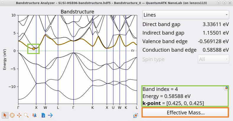
Let’s see how to estimate effective mass of electrons in bulk Si from the band structure calculated with the hybrid HSE06 functional. The EffectiveMass of holes and electrons can be estimated by fitting a parabola to the minimum/maximum of the conduction/valence bands.
Go to the Data View tool.
In the Data Sources, select the file Si-bandstructure-HSE06.hdf5 and then double-click on the Bandstructure_0 in the Data View window to open it with the Bandstructure Analyzer.
Find the lowest conduction band of Si and determine the minima. As shown in the image below, the minimum is located at k-point (0.425, 0, 0.425) with 0.585 eV energy, where 0.425 is 85% of the distance to the first Brillouin zone boundary at X=(1/2,0,1/2). At this point, the energy isosurfaces are ellipsoids, thus you get different values for the effective mass depending on if you look in the longitudinal (along) or transverse (perpendicular to Δ) directions.
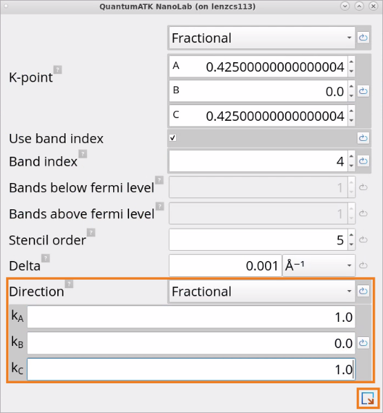
Click on the Effective Mass widget to open the Effective Mass block and set up an effective mass calculation at this conduction band minima k-point (0.425, 0, 0.425).
In the Effective Mass block, the parameters such as band index and k-point coordinates corresponding to the clicked point will be automatically set. Manually change the Direction to Fractional and set a=1, b=0, c=1, corresponding to the longitudinal direction.
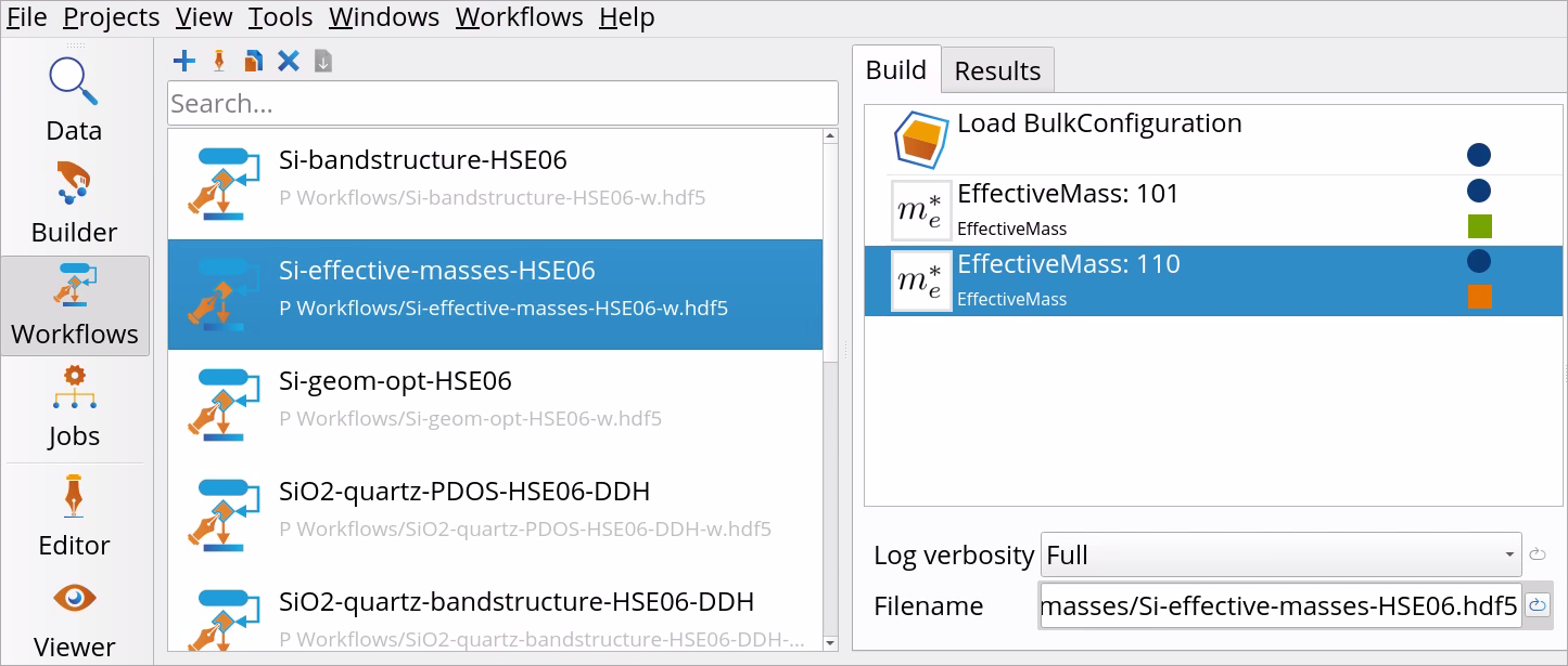
Click on the Send content to other tools button to add this calculation as a block to the Workflow located in the Workflow Area ‣ Build tab.
The workflow already has a Load BulkConfiguration block, which restarts the calculation from the former band structure calculation on Si: file Si-bandstructure-HSE06.hdf5.
Right-click on the Effective Mass block in the Workflow Area ‣ Build tab and choose to Duplicate the block.
In the duplicated Effective Mass block, change Direction to a=1, b=1, c=0, corresponding to one of the transverse directions.
Optionally right-click on Effective Mass blocks and choose to rename the blocks to Effective Mass: 101 and Effective Mass: 110, respectively.
Click on the Send content to other tools button and choose Jobs as a script to send the workflow to the Jobs tool in order to submit this job on a local machine or a remote cluster.
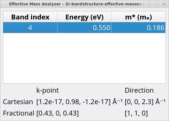
Once the calculation is finished, in the Data Sources, select the file Si-effective-masses-HSE06.hdf5 and then double-click on the EffectiveMass_0 and EffectiveMass_1 objects in the Data View window to open them with the Effective Mass Analyzer.
Here, the effective mass corresponding to the specified band and direction is reported. From the two EffectiveMass objects you will obtain:

 Workflow Builder, follow the step-by-step protocol described below. Here, you will use DFT with LCAOCalculator basis sets. For the DFT functionals, choose a hybrid HSE06 DFT functional for bulk Si (exact exchange fraction of 0.25 optimized for Si) and a dielectric dependent hybrid HSE06-DDH functional (DDHCustomExchangeCorrelation) for SiO2 (quartz) to find an improved material specific exact exchange fraction for more accurate band structure and band gap.
 Builder, click on the
  Send content to other tools button to send the optimized structures from the
  SetLCAOCalculator and Bandstructure blocks, respectively, to the middle Workflow Area ‣ Build tab.
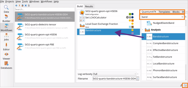
 Jobs tool in order to submit this job on a local machine or a remote cluster. It is recommended to parallelize over both MPI processes and threads in DFT simulations. Read the technical notes on Parallelization of QuantumATK calculations to learn more.
 Editor tool and then sent to the
  Data View tool.
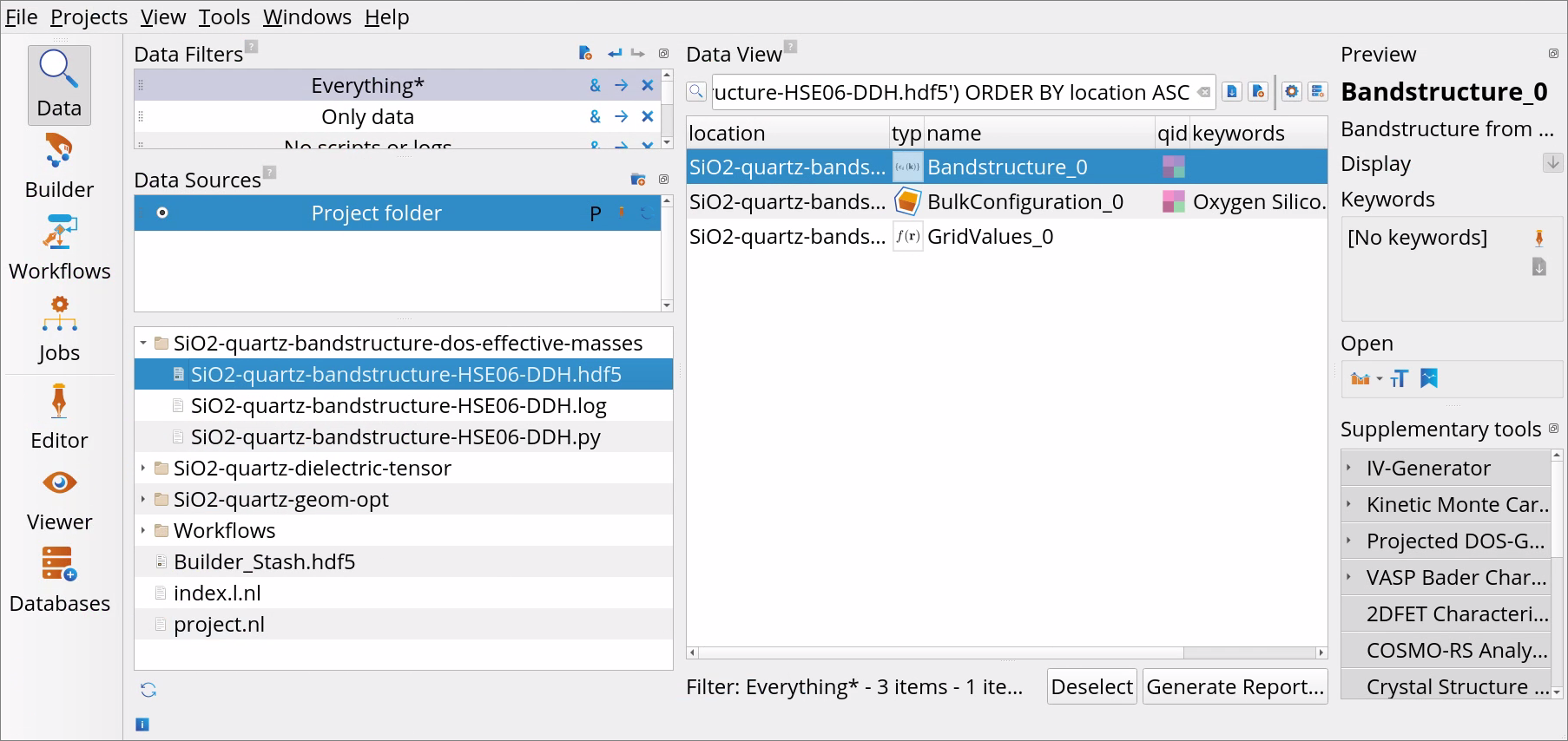
 Zoom and
  Plot editor tools and use measuring tools (right-click to Add measurement) to measure direct and indirect bandgaps yourself.
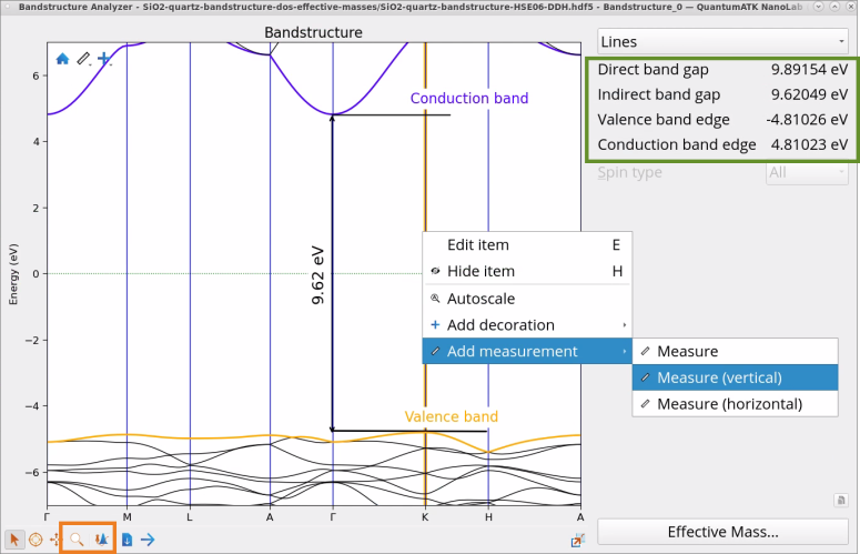
 Add button to add a new workflow.
 Load from file and ProjectedDensityOfStates blocks, respectively, to the middle Workflow Area ‣ Build tab.
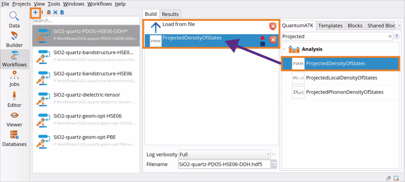
handle from the Projected DOS Analyzer to the Bandstructure Analyzer plot to combine the two plots.