GPU acceleration of proprietary feature calculations¶

DFT-LCAO, Semi Empirical, and Force Field calculations can be accelerated using GPU. Currently, NVIDIA GPUs are supported, for detailed requirements refer to the System Requirements.

Note

GPU acceleration of DFT-LCAO, Semi Empirical, and Force Field calculations is NOT supported on Windows. To take advantage of GPU acceleration, you must use the Linux version of QuantumATK.

This document describes how to run with GPU acceleration, which features are supported, and provide some guidance to attain best performance.

Enabling GPU acceleration¶

GPU acceleration of DFT-LCAO, Semi Empirical, and Force Field calculations is protected by a license key and it is not enabled by default.

There are alternative ways to request GPU acceleration:

Use the Job Manager and check the “Enable proprietary GPU acceleration” option in the Job settings, or when submitting your job.
Run the script (or interactive session) using the atkpython_gpu command instead of atkpython.
Set the environment variable QUANTUMATK_ENABLE_GPU_ACC=1 before running atkpython.

When GPU acceleration is requested the corresponding license will be checked out at startup. If the license key is not valid or the GPU is not supported, the program will exit with an error message. If GPU acceleration is enabled successfully, the log will display a message:

+------------------------------------------------------------------------------+
|                                                                              |
| GPU Acceleration                                                             |
|                                                                              |
+------------------------------------------------------------------------------+
| Compatible GPUs have been detected and proprietary CUDA acceleration has     |
| been enabled. All GPU features are supported.                                |
+------------------------------------------------------------------------------+

If compatible GPUs are detected but GPU acceleration was not requested, a warning is shown and DFT-LCAO, Semi Empirical, and Force Field calculations calculations will run on CPU.

Note

At startup a number of GPU licenses equal to the number of GPUs requested on the system by the user. The number of GPUs is determined by their unique IDs. If MIG (Multi Instance GPU) is enabled, each instance will be counted as a separate GPU.

LCAOCalculator and SemiEmpiricalCalculator¶

LCAOCalculator and SemiEmpiricalCalculator update is accelerated when the density matrix is calculated by direct diagonalization (default, see DiagonalizationSolver). Both non-distributed (processes_per_kpoint=1) and distributed (processes_per_kpoint>1) calculations are supported.

The speedup is more visible for calculation where most of time is spent in the diagonalization step, that is larger systems (100 atoms and above) and/or larger basis, Semi Empirical or DFT calculations with local functionals (LDA or GGA).

Hybrid functionals have a significant overhead and are only partially accelerated, therefore the speedup will be more moderate. ADMM projections are accelerated and can speed up significantly calculations for large systems.

There are no restrictions on the spin type, the GPU acceleration works for un-polarized, polarized, non-collinear and spin-orbit calculations.

Bulk Analysis¶

Bulk analysis objects which rely on direct or iterative diagonalization are accelerated, including:

Additionally, analysis object based on poisson solvers ParallelConjugateGradientSolver and NonuniformGridConjugateGradientSolver will also be accelerated, see dedicated section.

Other¶

All more complex workflows which requires frequent or heavy calculator update will be accelerated as a consequence of the calculator acceleration. This includes, among others:

Geometry optimization
Molecular dynamics
Nudged Elastic Band (NEB)
Defect calculations

DeviceLCAOCalculator and DeviceSemiEmpiricalCalculator¶

DeviceLCAOCalculator and DeviceSemiEmpiricalCalculator update is accelerated when GreensFunction method is selected as equilibrium_method or non_equilibrium_method (both, for best performance), and RecursionSelfEnergy as self_energy_calculator_real or self_energy_calculator_complex (both, for best performance). These are also the default settings, meaning that a default DeviceLCAOCalculator and DeviceSemiEmpiricalCalculator will use GPU acceleration.

Note

Only the serial version of GreensFunction is accelerated (processes_per_contour_point=1).

There are no restrictions on the spin type, the GPU acceleration works for un-polarized, polarized, non-collinear and spin-orbit calculations.

Device calculations can also use accelerated Poisson solvers, see dedicated section. In some cases, when the real space grid is fine and a large vacuum is present, that is for 1D and 2D systems, the Poisson solver can actually become the bottleneck, and the GPU acceleration of the Poisson solver can make a large difference.

The speedup is larger for systems with a large-cross section area, i.e. large number of atoms in the transverse directions (50 atoms or more) and/or large basis. More specifically, the speedup relates to the size of the blocks in the tridiagonal inversion algorithm [1]. For DFT calculations, the speedup is affected moderately by the choice of exchange-correlation functional. Hybrid functionals can exhibit a large speedup, because they lead to larger blocks in the tridiagonal structure.

Device Analysis¶

The most common device analysis objects are accelerated, including:

Additionally, analysis objects based on poisson solvers ParallelConjugateGradientSolver and NonuniformGridConjugateGradientSolver will also be accelerated.

IVCharacteristics¶

Since usually the most time consuming tasks of an IVCharacteristic calculation are the calculator self-consistent update and the transmission spectrum calculation, both of which are accelerated, the IVCharacteristic object can also show large speedup.

Poisson solvers¶

ParallelConjugateGradientSolver and NonuniformGridConjugateGradientSolver are GPU accelerated and can exhibit large speedup, especially DFT calculations which typically have many grid points. When either is used in a bulk or device calculator, the following analysis objects, which use the Poisson solver, are also accelerated:

Note that the FastFourierSolver and FastFourier2DSolver can be faster regardless of CUDA acceleration. However, ParallelConjugateGradientSolver and NonuniformGridConjugateGradientSolver support more boundary conditions, metallic and dielectric regions and are therefore commonly used for device simulations.

Force Field¶

Force Field simulations can be accelerated if the potential set contains at least one potential type which supports GPU acceleration. Potential types that can be accelerated are:

Long-range pair potentials
All coulomb solvers (real- and fourier-space)
Machine-learned Force Field (MTP and TorchX-based)

For details about GPU acceleration, please see the reference manual of the TremoloXCalculator.

Machine-learned Force Field Training¶

Training of machine-learned Force Field training using the MachineLearnedForceFieldTrainer can be accelerated with GPUs. This concerns primarily the training of MACE models based on the MACEFittingParameters.

Parallelization¶

GPU acceleration can be used together with MPI parallelization. There are no constraints on the number of MPI processes, and multi-node calculations are supported. The following recommendations apply:

Use a number of CPU cores proportionate to the number of GPUs on the node. For example, if you have 4 GPUs and 32 CPU cores, use 8 CPU cores per GPU. Otherwise, parts of the code which are not GPU accelerated could be slowed down significantly.
Using one MPI process per GPU, and threading to occupy the CPU cores, is a good starting point for most calculations. This is the setup which uses the least amount of GPU memory.
Calculations with multiple MPI processes per GPU are supported, and in some cases they can be faster. Note also that more GPU memory will be used, roughly proportionally to the number of MPI processes. In this case it is highly recommended to enable NVIDIA MPS (Multi Processing Service).

Performance tips for DFT and Semi-Empirical¶

System Size: Larger systems will have a larger speedup when compared to CPU calculations. This is because the overhead of the GPU is better amortized, and a larger fraction of the time is spent in the algorithms that are accelerated.
Bulk Systems:
- Use GPU acceleration for systems of about 100 atoms or more.
- For large systems, speedups of up to 10x can be achieved.
- The non-distributed diagonalization solver (processes_per_kpoint=1) is more efficient and should be preferred if GPU memory is sufficient.
- Typically, systems up to 1000 atoms or more can be run on a single GPU.
- For moderate-sized systems (100-1000 atoms), better performance might be achieved by using multiple MPI processes per GPU, if memory allows.
Device Systems:
- Acceleration depends on the structure of the tri-diagonal matrix (the larger the matrix blocks, the better the speedup), which is determined by:
  - Number of atoms
  - Cross-section size
  - Interaction length of the basis-set (or hamiltonian parametrization for Semi Empirical calculations)
- Parallelization tradeoffs: The optimal configuration depends on your specific system:
  - Medium-sized systems may benefit from multiple MPI processes per GPU for matrix operations
  - However, Poisson solvers achieve best speedup with a single process per GPU
  - Choose processes/threads based on whether your calculation is Poisson solver intensive or density matrix intensive
- Use the DevicePerformanceProfile object to obtain an initial estimate of performance and memory consumption for the density matrix calculation step, which is usually the bottleneck.

Examples¶

This section collects examples with timing comparison between GPU accelerated calculations and their CPU counterpart. Note that performance will depend on the specific hardware and software configuration, as well as the size of the system being simulated.

DFT bulk calculation¶

In this example we update self-consistently a Quartz supercell with 864 atoms, calculated with DFT using a GGA-PBE functional, the default Medium basis and 8 k-points. For CPU calculations, the fastest diagonalization solver was selected (optimize_for_speed_over_memory=True in DiagonalizationSolver).

The number of processes was chosen to maximize the number of concurrent k-point:

For the CPU calculation:

48 CPU cores: 8 processes 6 threads/process

For the GPU calculation:

1 GPU: 2 processes 6 threads/process (MPS enabled)
2 GPU: 4 processes 6 threads/process (MPS enabled)
4 GPU: 8 processes 6 threads/process (MPS enabled)

The results are shown in figure below: a single GPU is 2x faster as the full CPU node and the full GPU node is 10x faster than the full CPU node.

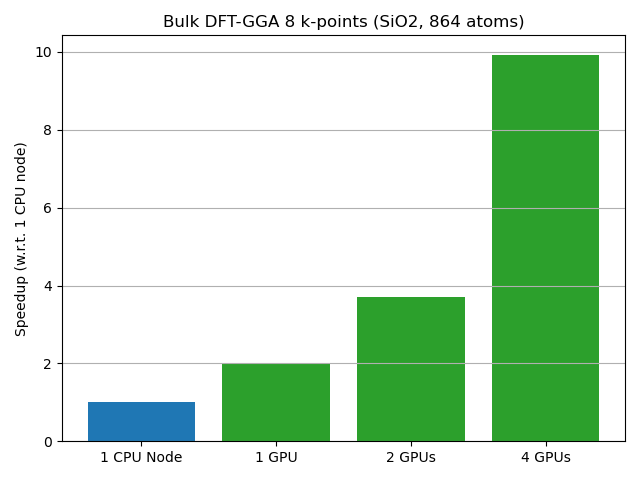
All calculations are executed on the same node (with GPU enabled or disabled), equipping 4 NVIDIA A100 with NVLink interconnect, and a two AMD EPYC 7F72 24-Core CPUs (48 cores total).

Geometry optimization¶

When running a geometry optimization, the largest computational cost is the calculator update. Therefore, the GPU speedup is close to what can be obtained for a self-consistent calculation.

This example is a geometry optimization of a GaN supercell with 768 atoms, using DFT with GGA-PBE functional, PseudoDojo High basis set and default k-point sampling. For CPU calculations, the fastest diagonalization solver was selected (optimize_for_speed_over_memory=True in DiagonalizationSolver).

The following table shows the total time for the CPU and GPU calculations.

	Turnaround time	Speedup
CPU Node	1d 12h 39m	1
GPU Node	4h 44m	7.74

CPU calculations were performed on an Intel Xeon IceLake node with 56 cores, using 4 MPI processes and 14 threads per process. GPU calculations were performed on 4 NVIDIA A100.

Device calculation¶

This example is a NEGF calculation of a High-K metal gate stack, using DFT and a hybrid functional (HSE06). The evaluation of the density matrix via GreensFunction is accelerated. Since hybrid functionals lead to long range interactions and dense hamiltonian blocks in the transverse direction, the speedup can be significant even for systems with a relatively small cross-section in terms of number of atoms and basis function.

The results are shown in figure below: a single GPU is as fast as a full CPU node, for a system with 916 atoms.

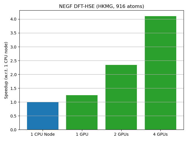
CPU calculations were performed on an Intel Xeon IceLake node with 56 cores, using 8 MPI processes and 7 threads per process. GPU calculations were performed on 4 NVIDIA A100, with 2 MPI processes per GPU and MPS enabled.

For larger cross-sections, even larger speedups can be achieved. On a system with twice the extension in the transverse direction (3364 atoms), speedup up to 9x can be achieved. However, GPUs with large amount of memory (80GB or more, e.g. H100) are required to run such calculation.