Electronic structure of NiO with DFT+U

Version: X-2025.06

Downloads & Links

NiO.py
NiO_DFT-script.py
NiO_DFT-WF.hdf5
NiO_DFT_results.hdf5
NiO_DFT_U-script.py
NiO_DFT_U-WF.hdf5
NiO_DFT_U_results.hdf5
NiO_DFT_abU-script.py
NiO_DFT_abU-WF.hdf5
NiO_DFT_abU_results.hdf5

Density Functional Theory (DFT), particularly in its standard forms like LDA or GGA, tends to underestimate the Coulomb interaction among localized d or f electrons. This leads to inaccurate predictions of electronic properties in strongly correlated systems, such as transition metal oxides, where the band gap is often significantly smaller than experimental values. To address this limitation, the DFT+U method introduces an empirical Hubbard U parameter that enhances the localization of d or f electrons. This correction improves the accuracy of band gap predictions, density of states (DOS), and defect level positions in materials with strong electron correlation or partial metallic character.

In this tutorial, we use NiO as an example of a typical strongly correlated material to demonstrate how to apply the DFT+U method in QuantumATK. Note that the projected density of states (PDOS) functionality was already introduced in the intro tutorial, so here we focus specifically on how DFT+U modifies the electronic structure.

Prerequisites

• Tutorial Band Structure, Projected Density of States and Effective Mass Calculations

Introduction

The self-interaction error is probably the most serious drawback of the LDA and GGA approximations to the exchange-correlation energy. This self-interaction can be described as the spurious interaction of an electron with itself. It has two main consequences:

• Electrons are over-delocalized;

• Band gaps in semiconductors and insulators are predicted to be much lower than their real counterpart.

The mean-field Hubbard correction, popularly called DFT+U, is a semi-empirical correction which tries to improve on these deficiencies.

In the DFT+U an additional energy term,

\[E_{U} = \frac{1}{2} \sum_\mu U_\mu \left( n_\mu - n^2_\mu \right),\]

is added to the Exchange-correlation energy [1]. In this equation, \(n_\mu\) is the projection onto an atomic shell and \(U_\mu\) is the value of the “Hubbard U” for that shell. The \(E_{U}\) energy term is zero for a fully occupied or unoccupied shell, while positive for a fractionally occupied shell.

The energy is thereby lowered if states become fully occupied. This may happen if the energy levels move away from the Fermi Level, i.e. increasing the band gap, or if the broadening of the states is decreased, i.e. the electrons are localized. In this way, the Hubbard U improves on the deficiencies of LDA and GGA.

The NiO crystal has a too low band gap in LDA and GGA and is one of the standard examples of how the DFT+U approximation can be used to improve the description of the electronic structure of solids [2]. In this tutorial you will compare the DFT and DFT+U models for this system using the GGA. You will both set the Hubbard U parameter manually and try set up an ab initio U model, where the U parameter is automatically and self-consistently calculated to then be used in a DFT+U calculation. This approach circumvents the tedious process of having to manually tune the U parameter for each atomic shell to fit to experimental or reference calculations.

Further details of the Hubbard U implementation in QuantumATK can be found in the manual: XC+U mean-field Hubbard term.

The electronic structure of NiO calculated with DFT

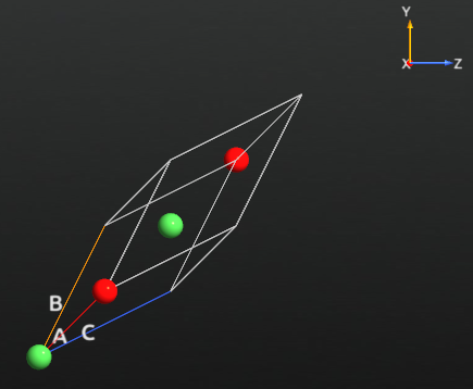
NiO has a fcc crystal structure with two atoms in the unit cell. The Ni atoms have a net magnetic moment and form an anti-ferromagnetic arrangement in the (111) direction of the fcc cell. The structure can be described by a rhombohedral unit cell with 4 atoms in the basis [1] as seen below. The script can be downloaded directly: NiO.py. It contains the structure of the crystal unit cell given in the QuantumATK ATK-Python format.

Note

The rhombohedral unit cell vectors are given as \(( 1,\frac{1}{2},\frac{1}{2}) a\), where \(a\) is the fcc lattice constant. The length of the rhombohedral unit cell vectors are therefore given by \(\sqrt{\frac{3}{2}} a\), and are in accordance with the experimental fcc lattice constant of 4.17 Å [3].

Setting up the calculation

You will in this section set up a spin-polarized DFT calculation using the spin-polarized version of the generalized gradient approximation (SGGA) for the NiO electronic structure and calculate the Mulliken population and the projected density of states(PDOS). If you are not familiar with the workflow of QuantumATK you are recommended to first go through the Introductory Tutorials. If you want to skip the setup you can download the final python NiO_DFT-script.py script, NiO_DFT-WF.hdf5 workflow and NiO_DFT_results.hdf5 result file.

Note

In general it is good practice to always optimize the geometry before running any electronic property calculation. However, for this specific system optimization was found to have insignificant influence on the results.

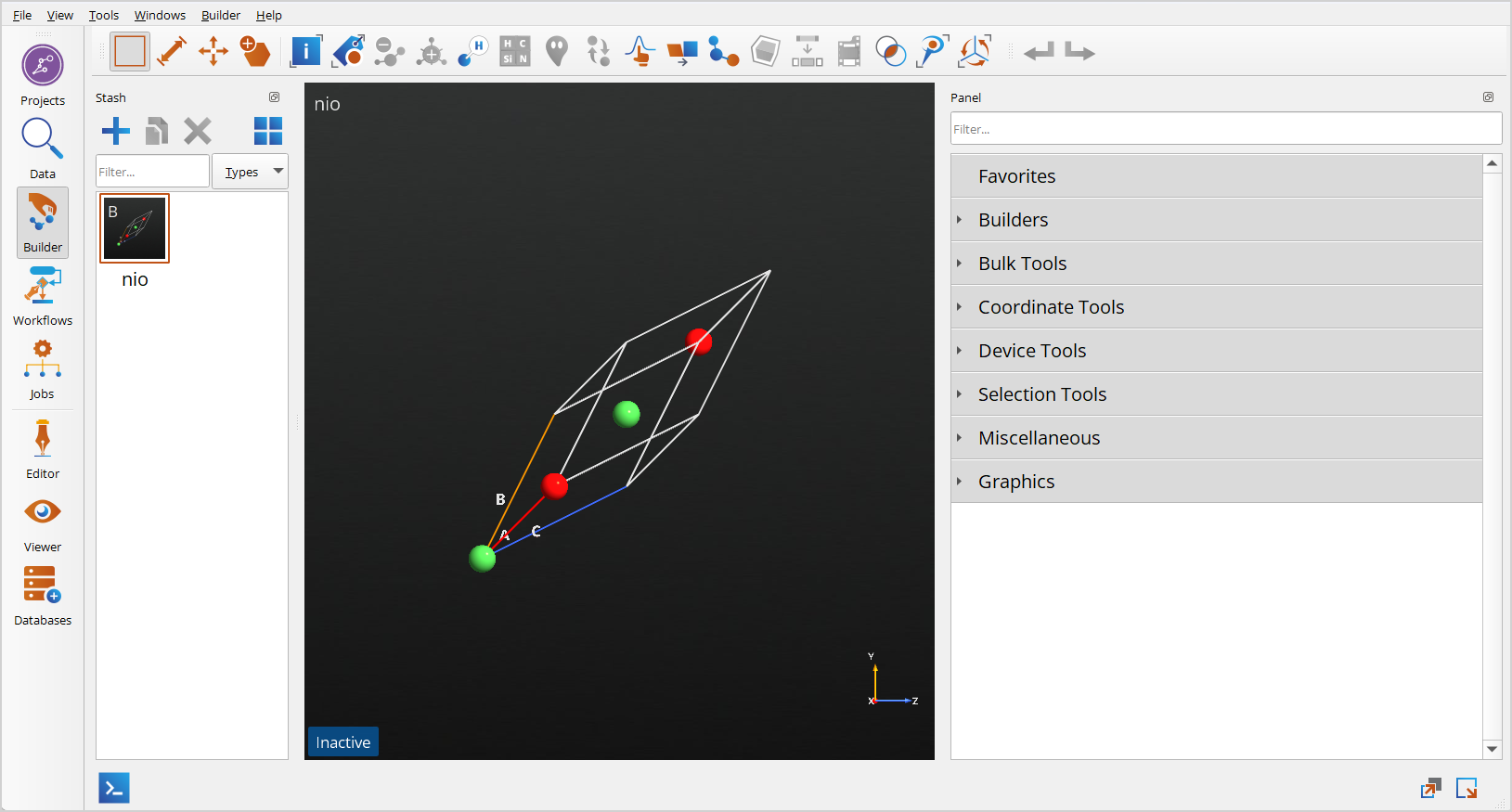
Start up QuantumATK and drag the script NiO.py onto the Builder. The NiO crystal will be added to the Stash.

Tip

Alternatively you can drag the script NiO.py directly onto the Workflows from the QuantumATK Project Files list.

Next, click the the button and select the Workflow Builder.

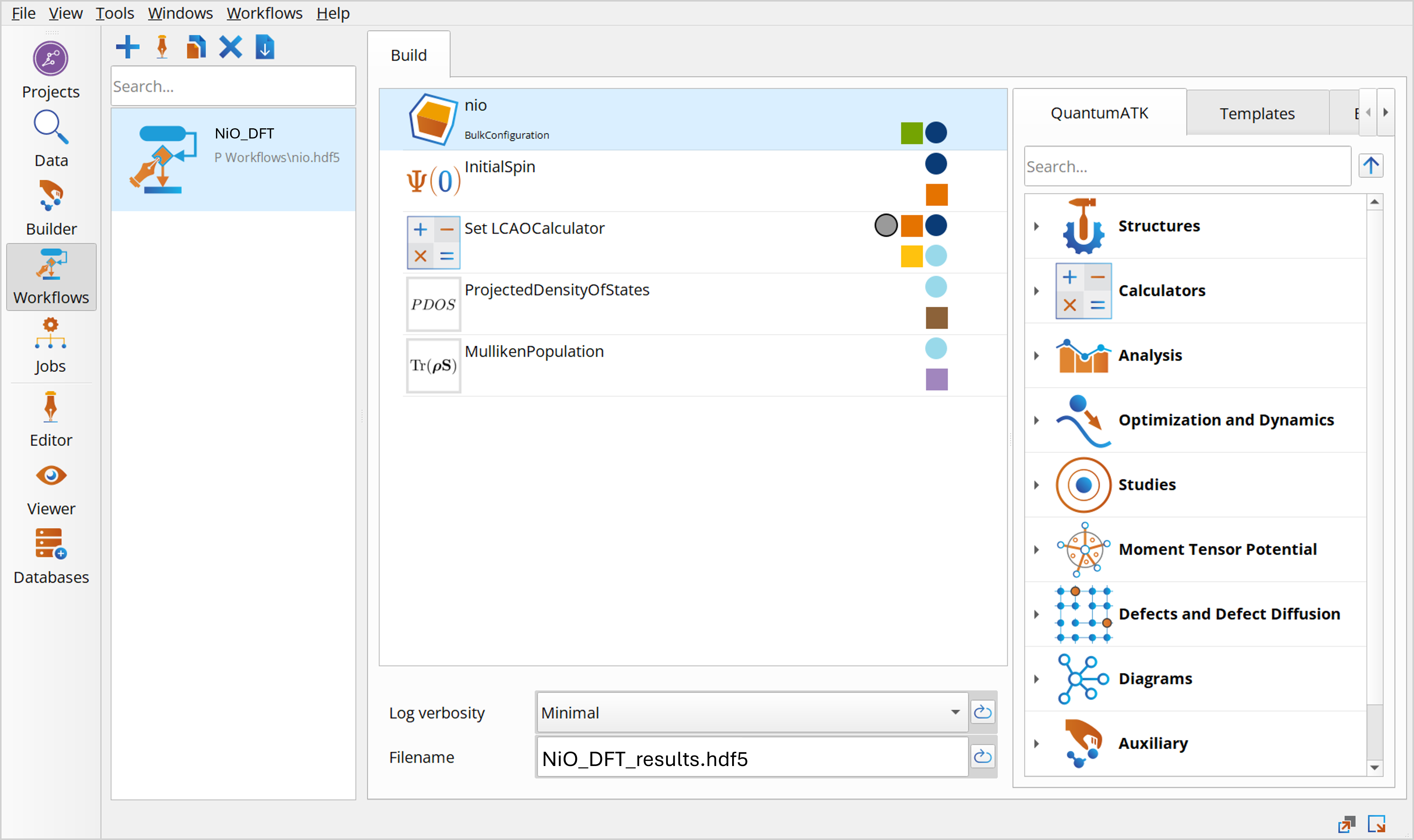
Change the default output file name to NiO_DFT_results.hdf5 and add the following blocks to the script:

• Auxillary ‣ Initial Spin

• Calculators ‣ Set LCAOCalculator

• Analysis ‣ ProjectedDensityOfStates

• Analysis ‣ MullikenPopulation

Note

It is important that the InitialSpin module is entered before the SetLCAOCalculator, otherwise the spin will be ignored.

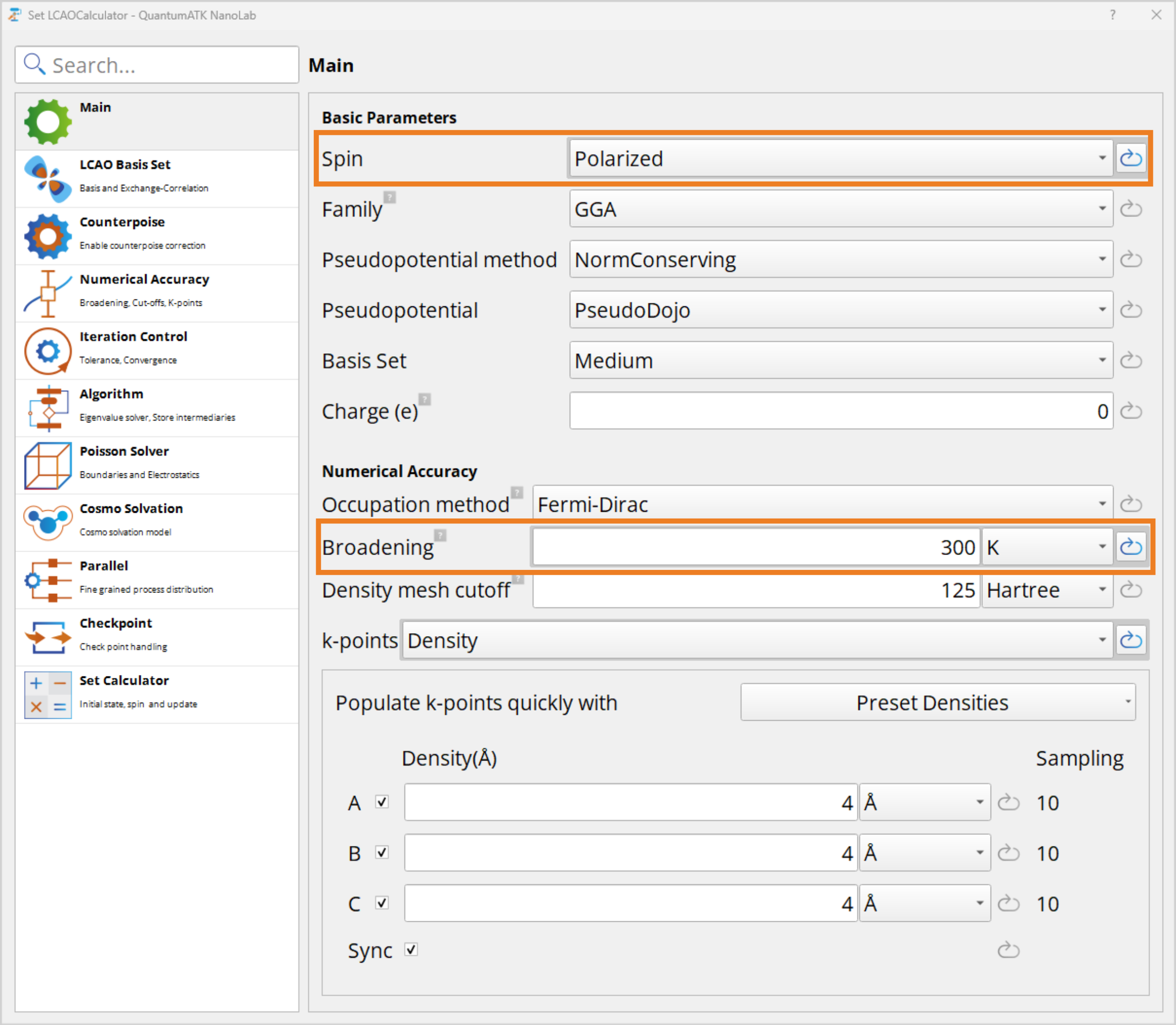
Now double-click the Set LCAOCalculator to open the calculator widget, and change the spin from Unpolarized to Polarized. Then change the Broadening to 300K, as it recommended for semiconductor materials. Under the Iteration Control the tolerance should be reduced to 1e-5 which is recommended for magnetic systems.

The next step is to set up the anti-ferromagnetic NiO spin arrangement. For this purpose, open the Initial Spin block.

By clicking the value of the Scaled spin, the spin can be set individually on each atom. Set opposite spins on the two nickel atoms and no spin on the oxygen atoms as illustrated below.

Important

The initial spin on each atom is given relative to the atomic spin of the element as obtained by Hund’s rule. For nickel the electronic configuration of the atom is \([\mathrm{Ar}]\,3d^8 4s^2\) (see element data in the manual - see Atomic data.). The 3d shell is fractionally occupied, and only this shell will contribute to the spin of the atom. According to Hund’s rule the 3d shell has 5 electrons in the up direction and 3 electrons in the down direction, giving a total atomic spin of 2\(\mu_B\) for nickel.

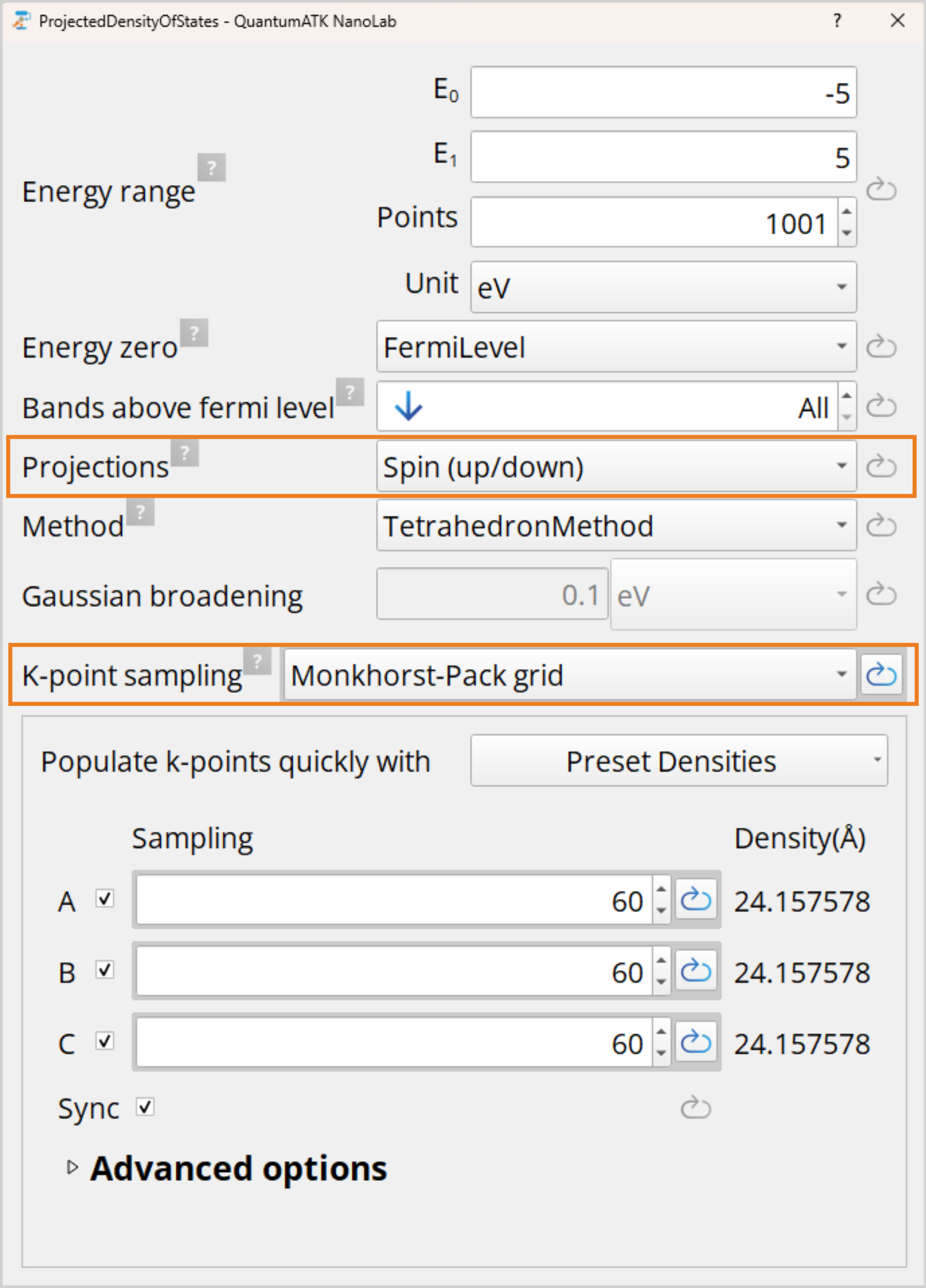
Finally, open the ProjectedDensityOfStates block and set Projections to Spin(up/down), this allows for the separation of the spin channels. A high k-point sampling is needed for sufficiently capturing fine details in the PDOS, thus change the K-point sampling from Default to Monkhorst-Pack grid and set 60x60x60 k-points.

Tip

You can set multiple Projections, however, each needs an individual block. Sites will allow to observe the projected DOS of each atom and Element will show the projected DOS of each atom type.

Save the current script by clicking Save the current file….

Performing the calculation

To start the calculation, send the script to the Job Manager by using the button.

The job takes about 11 minutes on a single node with 40 cores.

Analysing the results

To inspect the results go to Data View and locate the files.

Mulliken Population

To inspect the Mulliken population right click the MullikenPopulation hdf5-file and select Open with Text Representation. You will find a report as shown below.

+------------------------------------------------------------------------------+
|                                                                              |
| Mulliken Population Report                                                   |
|                                                                              |
+------------------------------------------------------------------------------+
|                        |                                                     |
| Element   Total  Shell | Orbitals                                            |
|                        |                                                     |
|                        |      s                                              |
|   0  Ni   9.243  0.997 |  0.997                                              |
|           7.850  0.997 |  0.997                                              |
|                        |      y      z      x                                |
|                  2.988 |  0.996  0.996  0.996                                |
|                  2.993 |  0.998  0.998  0.998                                |
|                        |     xy     zy  zz-rr     zx  xx-yy                  |
|                  4.898 |  0.987  0.987  0.968  0.987  0.968                  |
|                  3.500 |  0.981  0.981  0.279  0.981  0.279                  |
|                        |     xy     zy  zz-rr     zx  xx-yy                  |
|                  0.045 |  0.005  0.005  0.015  0.005  0.015                  |
|                  0.041 |  0.005  0.005  0.013  0.005  0.013                  |
|                        |      y      z      x                                |
|                  0.145 |  0.048  0.048  0.048                                |
|                  0.151 |  0.050  0.050  0.050                                |
|                        |      s                                              |
|                  0.169 |  0.169                                              |
|                  0.167 |  0.167                                              |
|                        |      y      z      x                                |
|                  0.000 |  0.000  0.000  0.000                                |
|                  0.001 |  0.000  0.000  0.000                                |
|                        | --------------------------------------------------- |

The Mulliken population reports the numbers of electrons per spin and orbital, as well as the orbital sum for each atom. Note that oxygen atoms are not polarized while the two nickel atoms are polarized in opposite directions, thus forming an anti-ferromagnetic arrangement. The polarization can be calculated from the difference between the number of electrons in the spin-up channel (9.243) and that in the spin-down channel (7.850). The resulting value of 1.39\(\mu_B\) is in good agreement with other DFT calculations using GGA [1], However, it is an underestimation of experimental results of 1.64 – 1.9\(\mu_B\) [4].

Projected density of states

To investigate the NiO projected density of states (PDOS), right click the ProjectedDensityOfStates item and select Open with Projected DOS Analyzer or simply double click the item. You can use Zoom to mark out the area of interest on the plot.

Tip

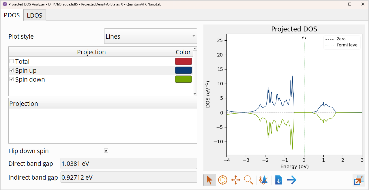
The plot shows the total projected density of states of the spin-up channel with a blue line and minus the result for the spin-down channel with a green line. If you select Flip down-spin in the Options menu, the density of states of the spin-down channel will be plotted on the negative axis.

The total Projected DOS shows no difference between the two spin channels. However, you saw from the Mulliken population that the nickel atoms are in fact spin polarized!

The calculation predicts a direct band gap of 1.04 eV and an indirect band gap of 0.93 eV, which is much smaller than the experimental value of 4.0 eV [4]. In the next chapter you will see how the description of the band gap is improved with the DFT+U approximation.

DFT+U calculation for the NiO crystal

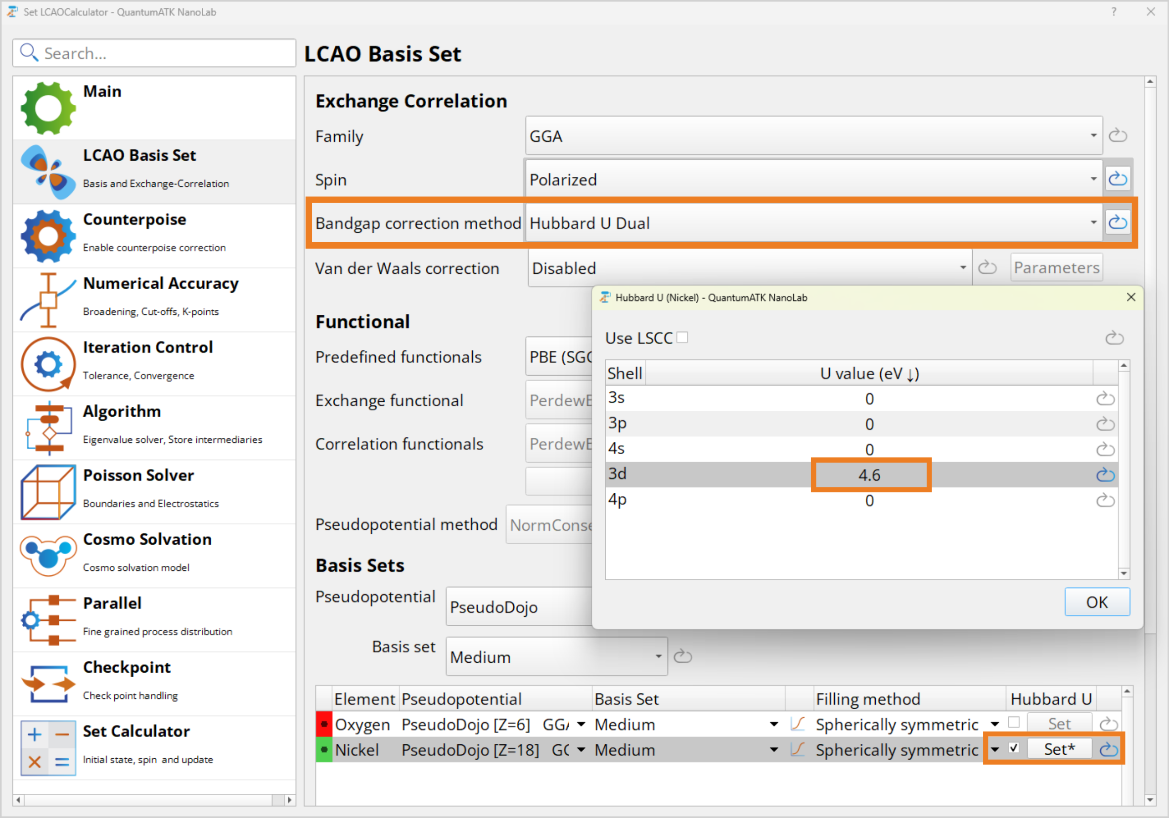
You will now perform a DFT+U calculation of the NiO crystal, using U = 4.6 eV for the nickle d-states. This U-parameter is taken from a study which fitted the value to provide a band gap in good agreement with experimental results [1]. You can also skip this by downloading the python NiO_DFT_U-script.py script, NiO_DFT_U-WF.hdf5 workflow and NiO_DFT_U_results.hdf5 results.

Calculations

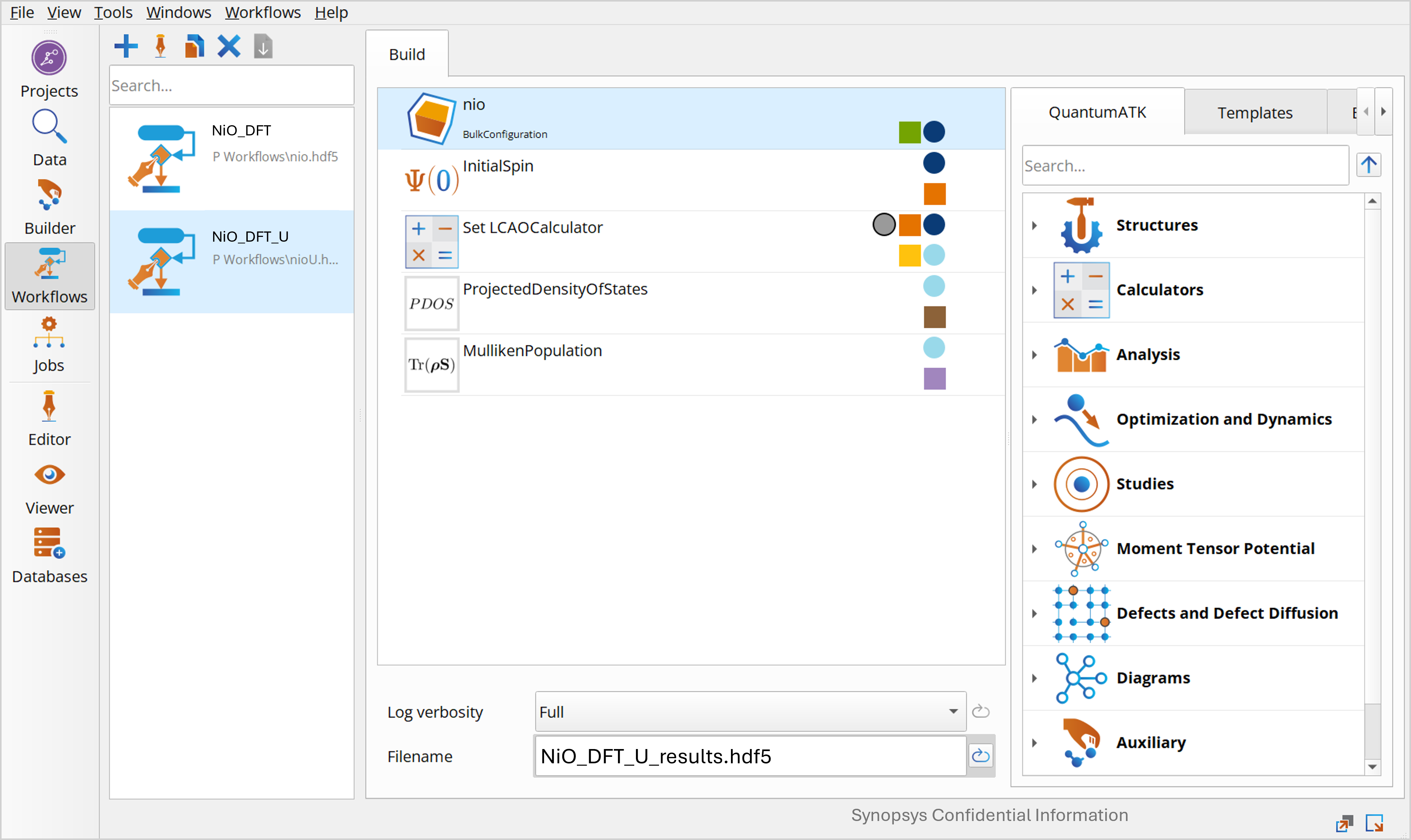
You will need to modify the script generated above for the SGGA calculation. Open Workflows again. Here you can right click the NiO_DFT workflow from before and select Duplicate, then rename the workflow NiO_DFT_U and change the output file name to NiO_DFT_U_results.hdf5.

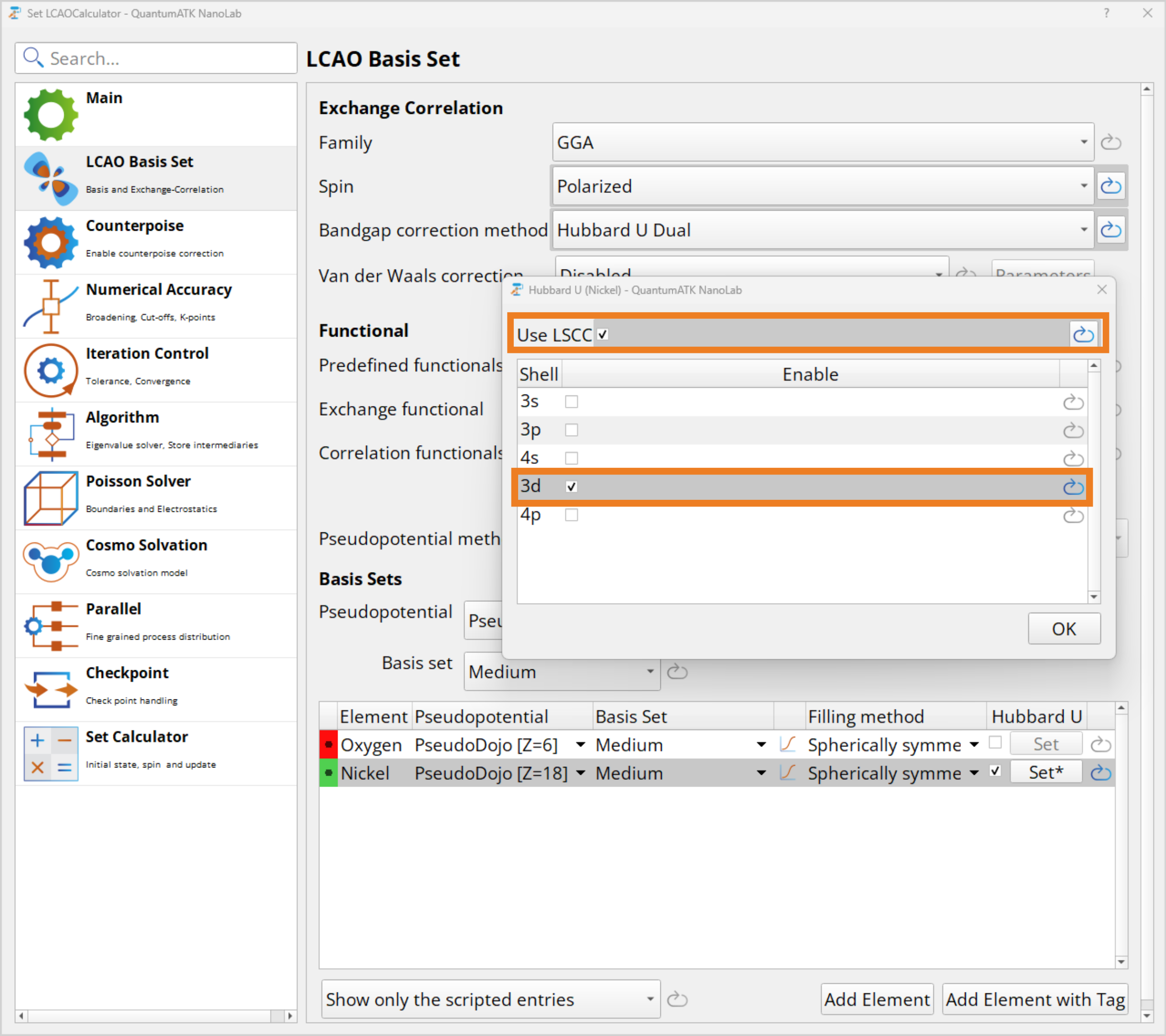
Open the set LCAOCalculator:

• In LCAO Basis Set, change Bandgap correction method to Hubbard U Dual. We choose Dual as it is the most realistic description of localized atomic orbitals we offer.

• Scroll down to the Basis Sets section and tick off the Hubbard U for Ni.

• Click Set* and set the Hubbard U parameter for the 3d orbital to 4.6 eV.

Next transfer the script to the Editor using the send to button, in order to check that all the parameters are properly set.

In the Editor locate the line where the nickel basis is defined and check that the Hubbard U parameter is set to 4.6 eV for the nickel_3d and nickel_3d_0 orbitals.

NickelBasis = BasisSet(
    element=PeriodicTable.Nickel,
    orbitals=[
        nickel_3s,
        nickel_3p,
        nickel_4s,
        nickel_3d,
        nickel_3p_0,
        nickel_3d_0,
        nickel_4p,
    ],
    occupations=[2.0, 6.0, 2.0, 8.0, 0.0, 0.0, 0.0],
    hubbard_u=[0.0, 0.0, 0.0, 4.6, 0.0, 4.6, 0.0] * eV,
    dft_half_parameters=Automatic,
    filling_method=SphericalSymmetric,
    onsite_spin_orbit_split=[0.0, 0.0, 0.0, 0.0, 0.0, 0.0, 0.0] * eV,
    pseudopotential=NormConservingPseudoPotential(
        "normconserving/pseudodojo/gga/standard/28_Ni.upf",
        local_potential_cutoff_threshold=1e-06 * Hartree,
        local_potential_cutoff_radius=6.0 * Bohr,
    ),
)

Now save the script as NiO_DFT_U_results.py and execute the job by sending it to Job Manager as before. This also takes around 11 minutes to run on a single node with 40 CPU cores.

Analyzing the results

First inspect the Mulliken population as before. You should find a magnetic moment of 1.72\(\mu_B\) on a nickel atom, which is in good agreement with the experimental result of 1.64 – 1.9\(\mu_B\) [4].

To determine the band gap, inspect the projected density of states as before. You should find that the projected DOS is zero in the range ~-1.70 to ~1.70 eV, and has a direct and indirect band gap of 3.32 and 2.88 eV respectively. This is much higher than values of ~1 eV for the non-corrected DFT calculation, and in better agreement with the experimental value of 4.0 eV [4].

Comparing the DFT and DFT+U projected DOS

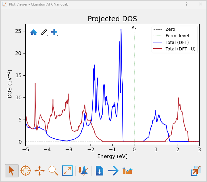
Now the PDOS obtained with DFT and DFT+U can be compared. From the Data viewer you can open the Projected DOS Analyser as before for both the DFT and the DFT+U calculations and use the drag and drop functions to merge the plots as described in the Band Structure tutorial.

Plotting the total projected DOS for both DFT and DFT+U clearly illustrates the large difference in band gaps between the two calculations (region of zero DOS around the Fermi level, at 0 eV energy).

Tip

• Naming the data sets before merging the plots makes it easier to keep track of which is which. The labels, colors and linestyles can be changed by clicking Edit

• The graph can be saved as a .hdf5 file, such that it can be edited later in Save or it can be exported as a picture by Export.

DFT + Ab initio U calculation for the NiO crystal

While the Hubbard U parameter improves the description of band gaps in correlated systems, it can be tedious to manually tune it for chosen orbitals. A more straight forward option is to use the DFT+ Ab inito U method, which is an effecient automatic self-consistent ab initio calculation based on Locally screen Coulomb Correction (LSCC) to obtain the Hubbard U parameter. You can find more information on the LSCC method in the manual: calculateLocalScreenedCoulombCorrectionHubbardU.

Tip

An alternative method for calculating the ab initio Hubbard U is the Finite Difference Linear Response approach. This technique computes U by evaluating the energy change resulting from variations in the occupation of localized d or f orbitals. While generally more accurate than the LSCC method, it is significantly more computationally demanding and is only available in Scripting. For details, see the manual: calculateFiniteDifferenceLinearResponseHubbardU.

Calculations

The set up is similar to the DFT+U calculation from before. However, this time when setting the Hubbard U parameter in the LCAO calculator, make sure to tick off the Use LSCC box and still tick off the 3d orbital. For this calculation the Log verbrosity shuld be set to Full.

Again by sending this script to the editor, you can check that the Hubbard U is set to LSCC for the Nickle 3d orbitals. Finally, run the job which also takes about 11 minutes. This can again be skipped by downloading the python NiO_DFT_abU-script.py script, NiO_DFT_abU-WF.hdf5 workflow and NiO_DFT_abU_results.hdf5 results.

Note

The LSCC method assumes that the Hubbard U energy is based on projections onto local basis set orbitals. While this specific projection is not implemented in QuantumATK, the Dual option offers the closest approximation. We advise against using the Onsite projection with LSCC-derived U values, as its orbitals differ significantly from those used in the LSCC calculations.

The Hubbard U values obtained via the LSCC method are highly sensitive to the choice of pseudopotentials and the shape of the basis set orbitals. As a result, these U values are not transferable between setups. Their reliability should be assessed based on how well they reproduce physical properties in actual DFT+U calculations.

In non-isotropic systems with many atoms, the Hubbard U values can vary between atomic sites. To assign different U values to individual atoms in a DFT+U calculation, each atom must be associated with a distinct basis set object. This is achieved by tagging each atom and assigning a specific basis set to each tag. You can automate this process using the utility function createLocalDFTUBasisSet(), as described in the LSCC manual: calculateLocalScreenedCoulombCorrectionHubbardU.

Analyzing the results

By double clicking the .log file you can find the Hubbard U which the calculation found and applied.

+------------------------------------------------------------------------------+
| Calculated LSCC U values (in eV)                                             |
| l = Thomas Fermi screening length (in Angstrom)                              |
+------------------------------------------------------------------------------+
|   0   Ni   (l=0.25)  3d: 9.52  3d:  3.2                                      |
|   2   Ni   (l=0.25)  3d: 9.52  3d:  3.2                                      |
+------------------------------------------------------------------------------+

Note

The two 3d orbitals correspond to different radial functions in the basis set:

• The first 3d orbital represents the valence-like 3d orbital from the atomic solution and receives a Hubbard U correction to account for electron correlation in the occupied states.

• The second 3d orbital is a more diffuse, “3d-like” virtual orbital, added to improve the flexibility of the basis set. It also receives a U correction to ensure consistent treatment of all 3d character in the system.

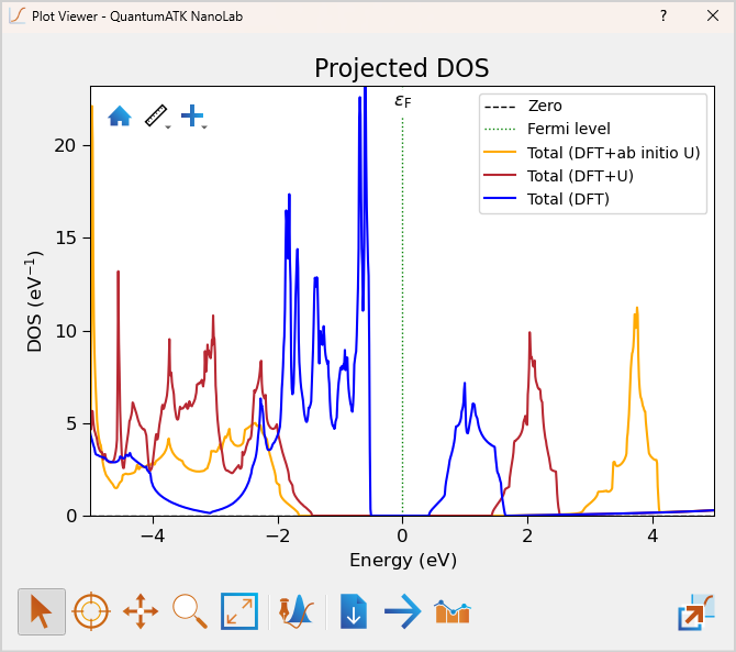
Merging the plot of the total projected DOS with the combined plot from before, the DFT+ Ab initio U is seen to further increase the indirect band gap from 2.88 eV (of the DFT+U) to 3.30 eV and the direct band gap from 3.32 eV to 3.92 eV. This is slightly closer to the experimental value of 4 eV [4] than using the fixed U=4.6 eV.

Final Remarks

In conclusion, GGA is found to severely underestimate the band gap of NiO with a direct and indirect band gap of 1.04 eV and 0.93 eV respectively. Using a fixed Hubbard U value, of 4.6 eV, the direct and indirect band gap is significanty improved to 3.32 eV and 2.88 eV respectively, coming closer to experimental value of 4.0 eV. In this case the self-consistent LSCC method further improves the band gap, yielding a direct and indirect band gap of 3.92 eV and 3.30 eV respectively.

Band Gap Comparison
Band Gap	no U	U=4.6 eV	LSCC
Direct	1.04 eV	3.32 eV	3.92 eV
Indirect	0.93 eV	2.88 eV	3.30 eV

References

[1] (1,2,3,4)

M. Cococcioni and S. de Gironcoli. Linear response approach to the calculation of the effective interaction parameters in the LDA+U method. Phys. Rev. B, 71:035105, Jan 2005. doi:10.1103/PhysRevB.71.035105.

[2]

A. B. Shick, A. I. Liechtenstein, and W. E. Pickett. Implementation of the LDA+U method using the full-potential linearized augmented plane-wave basis. Phys. Rev. B, 60:10763–10769, Oct 1999. doi:10.1103/PhysRevB.60.10763.

[3]

H. Benzerouk, F. Chouit, M. Mekhnache, L. Saad Hamideche, and A. Drici. An experimental and theoretical study of nickel oxide (nio) using the spraying method (csp) and dft calculations. Materials Science and Engineering: B, 303:117323, 2024. URL: https://www.sciencedirect.com/science/article/pii/S0921510724001521, doi:https://doi.org/10.1016/j.mseb.2024.117323.

[4] (1,2,3,4,5)

Vladimir I Anisimov, F Aryasetiawan, and A I Lichtenstein. First-principles calculations of the electronic structure and spectra of strongly correlated systems: the LDA+U method. Journal of Physics: Condensed Matter, 9(4):767, 1997. doi:10.1088/0953-8984/9/4/002.