Green’s function surface calculations

Version: 2016.0

This tutorial introduces you to a very novel method for computing surface properties: Green’s function surface calculations. The central difference to traditional slab calculations is that the surface electronic structure is coupled to the bulk electronic structure through the non-equilibrium Green’s function (NEGF) method.

The system you will investigate is a silver (100) surface, for which you will compute the work function. In particular, you will:

• construct the surface configuration;

• set-up and run the Green’s function surface calculation;

• analyze the work function and compare to results from traditional slab calculations.

Atomistic models of a surface

This section aims to introduce the Green’s function surface configuration, and compare it to the conventional slab model. The two figures shown below illustrate the differences between the two.

The slab consists of a finite number of silver layers, surrounded be vacuum in both directions along the C-axis, so it really has two surface–vacuum interfaces. The Hartree difference potential, $\Delta V_\mathrm{H}$, is bulk-like in the middle of the slab, but changes near the slab–vacuum interfaces, and becomes constant in the vacuum regions.

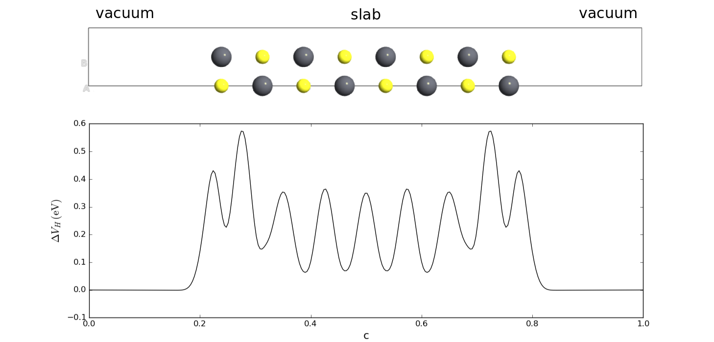
Fig. 117 The traditional slab model of a surface is surrounded by vacuum on both sides along the C-direction.

In contrast, the Green’s function surface model consists of a single surface region attached to an electrode (a fully periodic bulk). The electronic structure is matched at the electrode–surface boundary using Green’s functions. The surface is therefore electronically connected to a bulk substrate, and the surface chemical potential is fixed to that of the electrode.

Fig. 118 The Green’s function surface model has only a single surface–vacuum interface, and is geometrically and electronically connected to a periodic (bulk) electrode.

Advantages of NEGF

Green’s function surface calculations have some significant advantages over traditional slab approaches:

• The slab model is a finite system and it therefore has a finite number of electrons. Consequently, when transferring charge from a molecule to the surface (or the other way around), the total number of electrons will change, and therefore the chemical potential of the electrons in the slab also changes. This is a spurious effect, and the Green’s function surface model alleviates it completely by coupling the surface to an infinite reservoir of electrons at a fixed chemical potential (the electrode).

• Convergence of computed properties wrt. slab thickness is always an issue, and various corrections are ofte needed to avoid interactions with repeated images of the simulation cell. With the proper choice of boundary conditions, QuantumATK Green’s function surface calculations converge very easily wrt. surface thickness, as we shall see later in this tutorial.

NEGF calculation with a single electrode

As already mentioned, the Green’s function surface configuration consists of an electrode and a surface region (also called the central region). In the language of QuantumATK, it is therefore a device configuration with a single electrode. As in any QuantumATK device calculation (using NEGF), the calculation proceeds in two steps:

1. The electrode bulk electronic structure is calculated first. This is usually very fast.

2. The NEGF calculation then proceeds to calculating the ground state of the surface region only, given the constraint that the electronic structure at the electrode–surface interface must match.

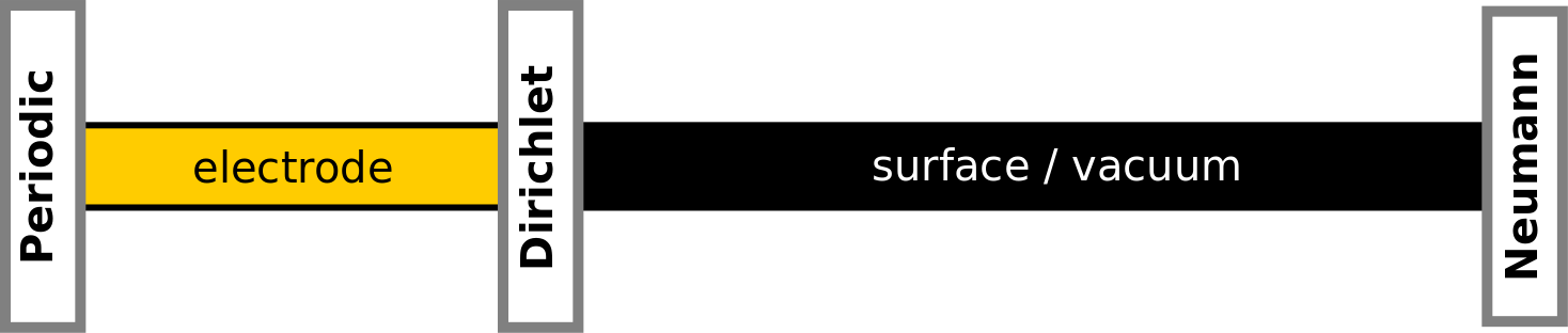
As illustrated below, three different sorts of boundary conditions are used along the C-direction of the simulation cell. The electrode ensures full periodicity towards the left, while a Dirichlet boundary condition is used at the electrode–surface interface. The Neumann boundary condition is then the natural choice on the right-hand boundary.

Work function of Ag(100)

You will now calculate the work function of Ag(100) using DFT and Green’s functions. The basic workflow is this:

1. Use the Builder to construct the surface configuration from a stress-optimized silver bulk, and specify ghost atoms.

2. Use the Scripter to create a script that calculates the ground state, and saves the Hartree difference potential (HDP) and chemical potential.

3. Use the 1D Projector tool to visualize the HDP.

4. Calculate the work function from the HDP and chemical potential.

Build the surface configuration

You will first need to cleave a silver bulk configuration along the (100) direction. To this end, you will use a silver bulk optimized at the LDA level using FHI pseudo-potentials and a SingleZetaPolarized basis set.

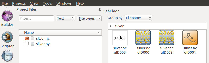
Create a new QuantumATK Project, and download a HDF5 file containing the optimized structure: silver.hdf5. Save it in the Project Folder such that its contents become visible on the LabFloor. You will notice that the silver silver band structure was also calculated – this will prove useful later on. You can also obtain the script used for the calculations: silver.py.

Tip

You may refer to the tutorials Geometry optimization: CO/Pd(100) and Calculate the band structure of a crystal for more information on how to perform a bulk geometry optimization and a band structure calculation.

From the LabFloor, transfer the relaxed silver bulk configuration (object id gID002) to the Builder and confirm that the optimized LDA-SZP lattice constant is 4.148 Å. Then select the configuration and open the Builders ‣ Surface (Cleave) tool.

This tool allows you to cleave the silver crystal along the (100) direction: Click Next twice, and choose the “Non-periodic and normal (slab)” output configuration with 10 metal layers, as illustrated below.

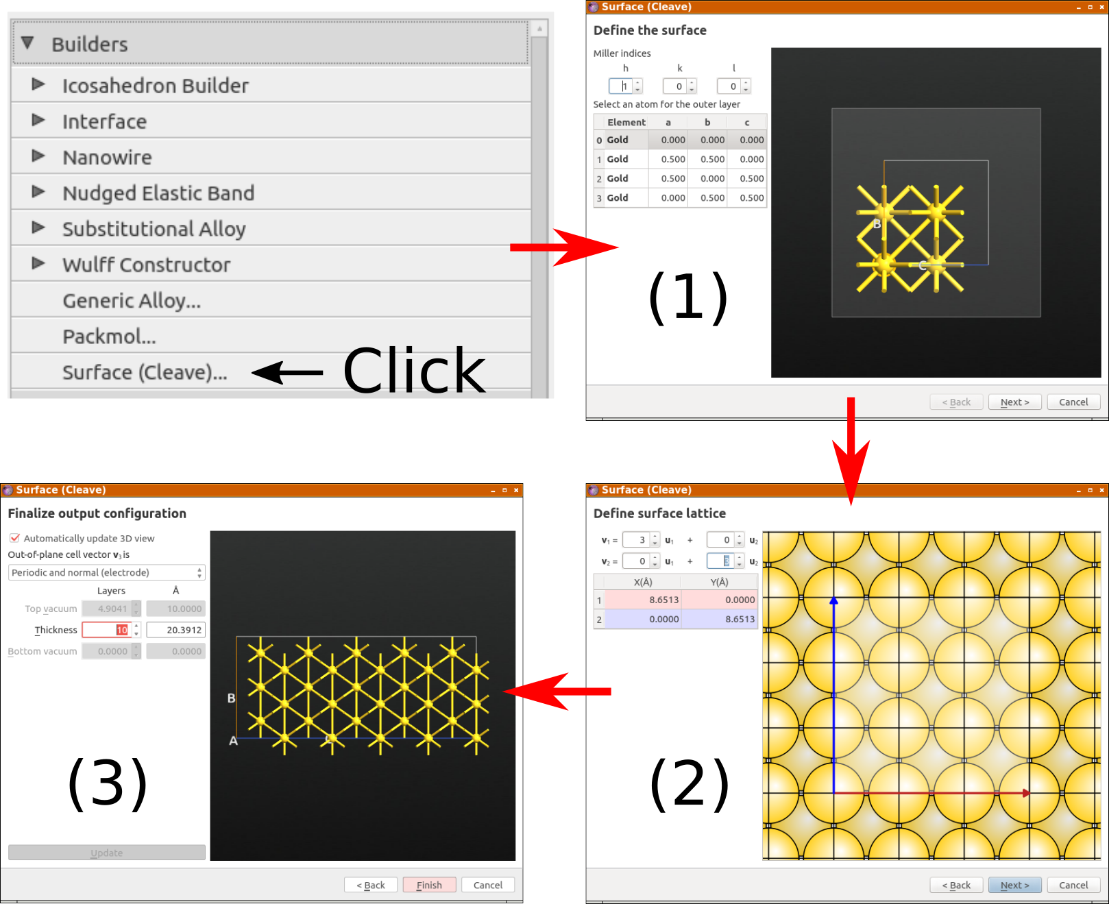
The item silver.hdf5 (100) is now in the Stash. Select it and use the Device Tools ‣ Surface From Bulk to create the surface configuration needed for the Green’s function surface calculations.

The Surface from Bulk widget allows you to select the size of both the electrode and the surface (here denoted the central region). The default electrode length of 8.3 Å will do just fine. Note that you can also change the size if the central region attached to the electrode.

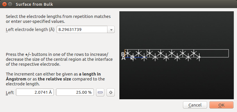
Click OK to add the configuration to the Stash. The name of the new item is automatically prefixed Surface.

Ghost atom

As discussed in the tutorial Computing the work function of a metal surface using ghost atoms, accurate work function calculations with a localized basis set require one or more ghost atoms immediately above the surface. This is most easily accomplished by turning the top-most atom into a ghost atom.

Select the top-most atom as shown in the image below, and click the icon in the top panel bar.

The atom is now designated a ghost atom, i.e. a basis set center with no nucleus.

Transfer the surface configuration to the Script Generator using the icon, and proceed to the next section to set up and run an QuantumATK script for the Green’s function surface calculation.

Calculations

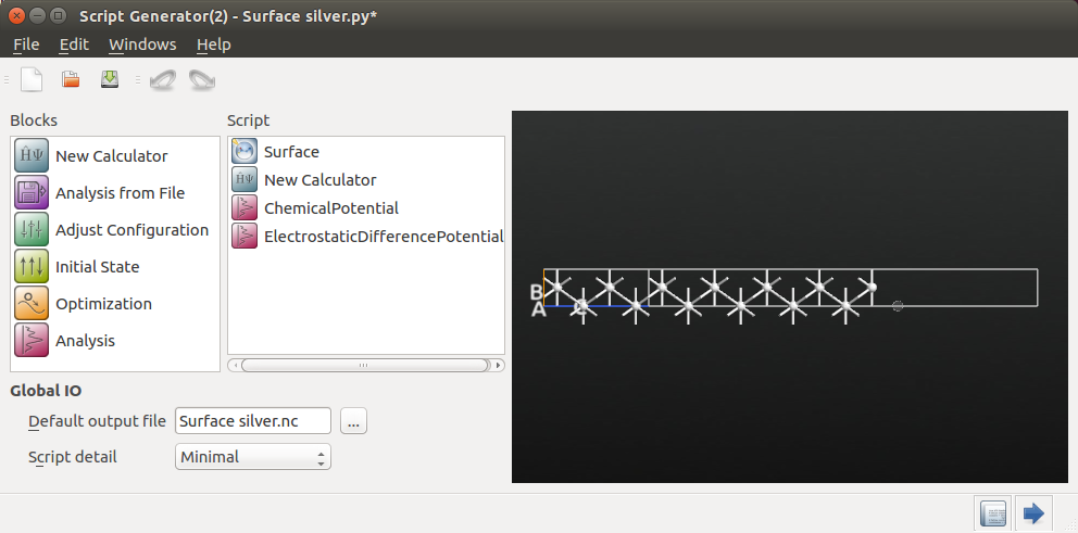
The Script Generator is a graphical interface for writing an QuantumATK Python script. Add the following blocks to the script by double-clicking them:

• New Calculator.

• Analysis ‣ ChemicalPotential.

• Analysis ‣ HartreeDifferencePotential.

Then double-click the added New Calculator block to open it. In the Basic device calculator settings, choose LDA exchange-correlation and a 9 x 9 x 100 k-point grid.

Note

As discussed in detail in the introductory tutorial Transport calculations with QuantumATK, it is vital to use a relatively large number of k-points along the C-direction in QuantumATK device calculations, e.g. 100. Importantly, these are only used in the electrode calculation, which is relatively cheap to calculate, and are not used in the main part of the QuantumATK device calculation: The central region is by definition not periodic along C, so it has only a single k-point along C.

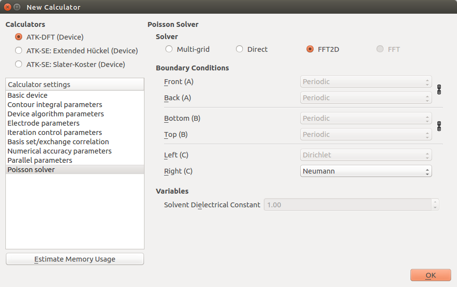
Next, navigate to the Basis set/exchange correlation settings, and choose the SingleZetaPolarized basis set. Lastly, in the Poisson solver settings, change the boundary condition on the right-hand C-face to Neumann.

Contour integral

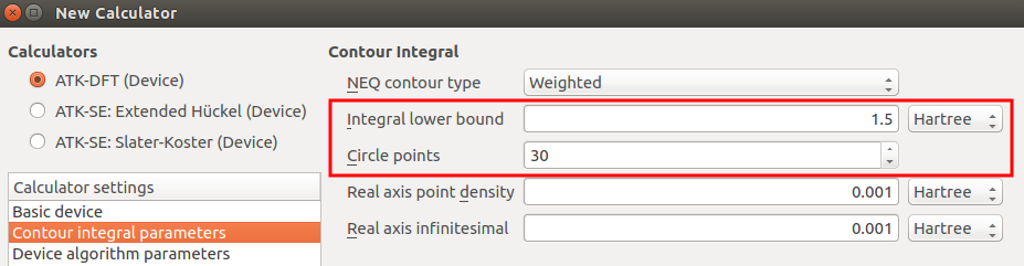
The NEGF method uses a contour integral to evaluate Green’s functions. As explained in anothor tutorial (Finite-bias calculations), the default values for the settings Integral lower bound and Circle points may need to be increased if the applied pseudopotentials have deep-lying (semi-core) states.

It is therefore good practice to check the electrode band structure, in order to make sure that the lowest band does not fall outside the lower bound on the contour integral. In the present case, we can use the silver band structure stored in the file silver.hdf5, which is illustrated below.

The deepest energy eigenvalue is band is 7.8 eV (0.29 Hartree) below the Fermi level, which is well within the default contour integral energy window (1.5 Hartree below the Fermi level). No need to increase the lower bound, so you should just stick to the default value.

Save the script and run it

Back in the Script Generator main window, change the default output file name silver_gfs.hdf5 and save the Python script as silver_gfs.py. If needed, you can also download the final script: silver_gfs.py.

Then execute the script using the Job Manager or from a Terminal. The calculation should take about 4 minutes on a laptop.

Analysis

Once the calculation is finished, the HDF5 data file silver_gfs.hdf5 arrives on the LabFloor. It contains the (one-probe) surface configuration with a converged calculator, and the ChemicalPotential and HartreeDifferencePotential (HDP) analysis objects:

One-probe surface configuration
ChemicalPotential
HartreeDifferencePotential

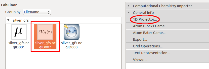
You should first take a look at the Hartree difference potential throughout the surface configuration. Use the mouse to select the HDP item, and then open the 1D Projector tool from the right-hand plugins panel.

The HDP is represented on a 3D grid, but the 1D Projector allows you to project it onto any unit cell axis. Project the average HDP onto the C-axis in order to get the visualization shown below.

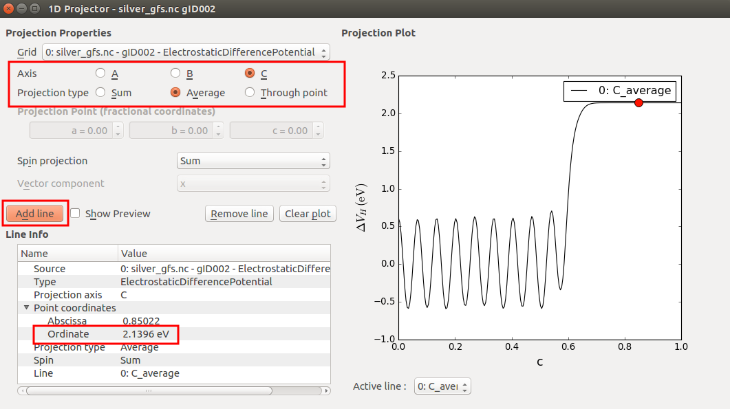
The Ag(100) work function is calculated from the difference between the (constant) Hartree difference potential in the vacuum region and the chemical potential (which in Green’s function surface calculations is really the chemical potential of the electrode):

$$\mathrm{WF} = \delta V_\mathrm{H}^\mathrm{c=1} - \mu$$

By moving the red dot in the projection plot to the far-right end, where c=1, you can read off $\delta V_\mathrm{H}^\mathrm{c=1}$= +2.14 eV.

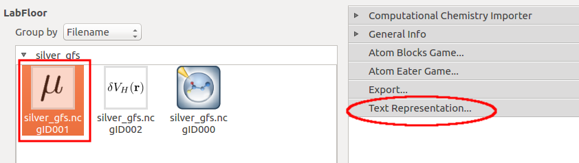
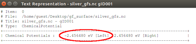
Next, use the Text Representation plugin to see the value of the chemical potential. You will find that $\mu$= –2.46 eV.

The theoretically predicted work function is therefore 4.6 eV, which is in very good agreement with the experimental value (4.64 eV). Note, however, that the top surface layers were not relaxed. You can easily do this by inserting the OptimizeGeometry block in the QuantumATK script.

Convergence wrt. metal layers

As a final illustration of the diference between Green’s function surface calculations and traditional slab calculations, the figure below shows how the predicted Ag(100) work function converges wrt. the number of silver metal layers. The Green’s function calculations are similar to the one done above, but one extra ghost atom is used.

It is quite clear that work functions computed using the Green’s function surface model converge much faster than those calculated with the traditional slab model.

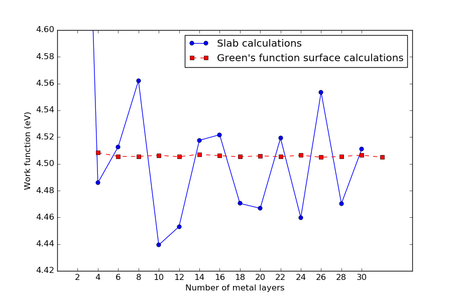
Fig. 119 Convergence of calculated Ag(100) work functions wrt. the number of metal layers. Work functions computed using the Green’s function surface model converge much faster than those calculated with the traditional slab model. For surface configurations, the number of metal layers includes the two electrode atoms.

If you like, you can reproduce the calculations using the scripts wf_slab.py and wf_surface.py, and plot the results using plot.py.