Computing the work function of a metal surface using ghost atoms
Version: 2017
In this tutorial you will learn how to compute the work function of a metallic surface using ATK. You will create a slab model of Ag (100) surface, use ghost atoms to improve the description of its electronic properties, and use the appropriate boundary conditions to describe correctly the presence of vacuum above it. It is assumed that you have some experience with ATK.
Why use ghost atoms?
Work function calculations depend critically on accurately simulating the decay of the surface charge density into vacuum, but short-ranged localized basis sets are sometimes not adequate for this. In this case, extra LCAO basis functions are positioned above the surface – these are called ghost atoms.
Setting up the geometry
In this section, you will set up a slab model of Ag(100) surface with ghost atoms, and calculate the work function of the surface.
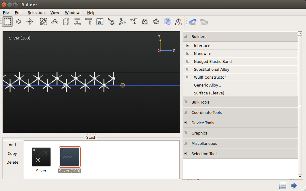
Open Builder (icon
 ). Click
, find “silver,”
and add it to Stash.
). Click
, find “silver,”
and add it to Stash.Open . Use Surface (Cleave) widget to define the surface by cleaving the bulk silver normal to the [100] direction.

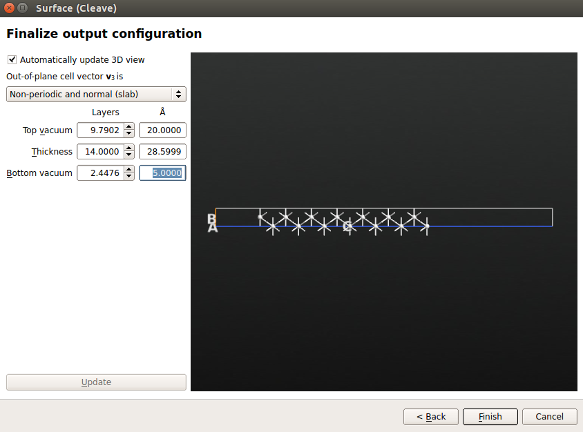
Click “Next” twice. On the final page of the Surface (Cleave) widget, set the out-of-plane cell vector v3 to be “Non-periodic and normal.” Set the rest of the parameters as follows:
Top vacuum = 20 Å. This large vacuum above the surface ensures that the effective potential has enough space to decay to the vacuum level.
Thickness = 14 layers.
Bottom vacuum = 5 Å. This vacuum ensures that no basis functions extend to the bottom edge of the cell (the radius of the basis functions for default silver is 3.7 Å).
Attention
This parameter setting ensures the convergence of work function.
Warning
In the direction normal to the surface, the non-periodicity of the system requires appropriate boundary conditions.
Click “Finish”. The surface structure will now appear in Stash.
To finalize the geometry setup, select the atom with the largest Z coordinate in Builder and turn it into a ghost atom by clicking the icon
 .
.As a result, the slab consists of 13 layers. The role of the ghost atom on the surface is to describe the smooth decay of electron density in the vacuum.
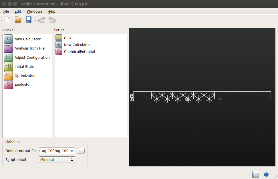
Send the structure to Script Generator (icon
 ).
).
Note
Changing an atom into a ghost atom means setting its potential, e.g., pseudopotential or nuclear charge there, to be zero. The basis functions are, however, still deployed there to describe the electron density. An alternative is to extend the range of the basis functions at every atomic position, although it makes the calculation expensive if the system is not as simple as in this example.
Defining the parameters of the calculation
In Script Generator, insert a New Calculator by double-clicking it in Blocks panel. Also, click to compute the chemical potential of the slab.
Note
Imposing appropriate boundary conditions at the top and bottom of the slab as shown below makes the chemical potential equal to the work function.
Set a suitable file name for the HDF5 file, e.g., “Ag_100.hdf5.”
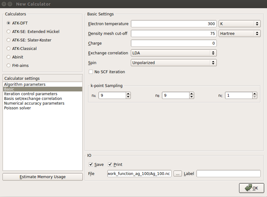
Double-click the New Calculator in Script panel and set the following parameters:
For accurate description of the electronic structure, set the k-point sampling to be 9x9x1 in Basic section of Calculator settings
Note
Remember in general to check the convergence of the properties of interest with respect to the fineness of the k-point grid.
In Basis sets/Exchange correlation section, select “SingleZetaPolarized” for the basis set.
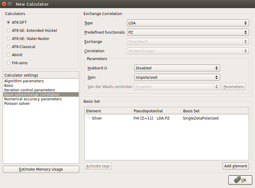
Note
Employing this basis set achieves good accuracy for this slab model with moderate computational effort. For other systems, however, it is not ensured that the use of the same basis set always provides enough accuracy.
Warning
Generally it is not advisable to use the TB09-MGGA to compute the work function, because the TB09-MGGA potential diverges in the vacuum. For the use of TB09-MGGA, the c-parameter should be tuned to obtain a reasonable value of the work function, and correct electronic structure of the material. In the present case, setting c = 0.94 gives WF = 4.44 eV, in excellent agreement with the LDA result (see below). Note that the value of c differs from that calculated self-consistently for bulk Ag, c = 1.31.
Finally, the most important setting: in Poisson solver section, select the Multi-grid Poisson solver. Then, click “chain” icon (marked in green in the picture below) to unlink the settings of the Left and Right cell boudaries, and set the Neumann boundary condition on the Left boundary, and the Dirichlet boundary condition on the Right cell boundary, respectively.
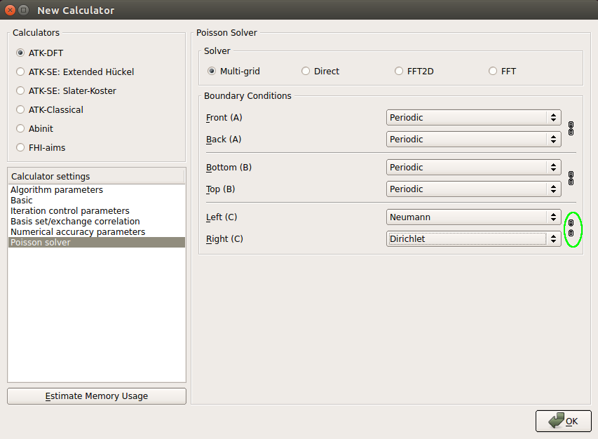
Note
Dirichlet boundary condition determines the Hartree potential to be zero on the right cell boundary, to mimic the presence of vacuum far away from the surface. Because of non-periodicity in the C direction, Neumann condition is used to demand the gradient of the Hartree potential to vanish on the left of the system.
Calculation and analysis
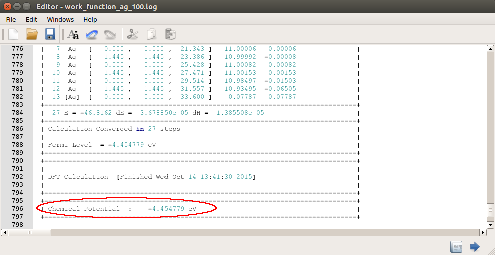
Send the structure to Job Manager and carry out the calculation. After the calculation, inspect the log file by clicking the
 button.
Around the end of the log file, the chemical potential, or the work function is printed. The value obtained for Ag 100 is 4.45 eV, which lies in the range from 4.22 to 4.81 eV, reported by experiments.
Just to demonstrate that with ATK it is also possible to get accurate results for other metals, see the comparisons with experiments in the table below:
Surface |
Measured WF (eV) |
WF calculated using the LDA (eV) [1] |
|---|---|---|
Ag (100) |
4.64 |
4.45 |
Ag (110) |
4.52 |
4.17 [2] |
Ag (111) |
4.74 |
4.71 |
Al (100) |
4.41 |
4.42 |
Au (100) |
5.28 |
5.38 [3] |
Ca (100) |
2.87 |
2.85 |
Cu (100) |
4.53-5.10 |
4.92 |
Li (100) |
2.93 |
3.14 |
Nb (100) |
3.95-4.87 |
3.95 |
Pb (100) |
4.25 |
3.95 |
Pt (100) |
5.12-5.93 |
5.97 |
Tl (100) |
3.84 |
3.74 |
W (100) |
4.32–5.22 |
4.01 |
Comments
Above we have commented in a few places on the importance of carefully checking convergence in certain numerical as well as geometrical parameters. The work function is quite sensitive to all of them, and so, for convenience, let us summarize the most important ones:
The script can be run in parallel using MPI for a considerable performance benefit, due to the large number of k-points, which is one of the parameters QuantumATK parallelizes well over.
By comparing the values reported in the table above for the (100), (110) and (111) crystalline faces of Ag, it appears clear that the work function depends on the crystalline face considered.
List of references:
A. W. Dweydari and C. H. B. Mee, physica status solidi (a) 27, 223 (1975)
M. Chelvayohan and C. H. B. Mee, J. Phys. C. Solid State Phys. 15, 2305 (1982)
CRC Handbook on Chemistry and Physics, pages 12-114 (2008)
J. K. Grepstad, P. O. Gartland and B. J. Slagsvold, Surface Science 57, 348-362 (1976)
J. C. Rivière, Appl. Phys. Lett. 8, 172 (1966)