Photocurrent in a silicon p-n junction
Version: O-2018.06
In this tutorial, you will learn how to calculate the photocurrent through a device under illumination. We consider a 7.6 nm sized silicon p-n junction, and showcase the Photocurrent Analyzer introduced with the QuantumATK O-2018.06 release.
The photocurrent is calculated by adding the electron-photon interaction to the device Hamiltonian,
using first-order perturbation theory, as described in [1] and in the ATK Manual:
Photocurrent.
Device ground state
At first you will perform the self-consistent device calculation. Then, using the ground-state device Hamiltonian, you will calculate and analyze the photocurrent.
You should use the script silicon_pn_junction.py to run the ground-state calculation –
both the doped device configuration and the appropriate NEGF calculator are defined in the script.
Results are saved in silicon_pn_junction.hdf5.
Simply download the script and run it using the  Job manager
or from a terminal. Once the calculation is done, you can see the file
Job manager
or from a terminal. Once the calculation is done, you can see the file silicon_pn_junction.hdf5
on the LabFloor. The calculation takes ca. 20 mins with 4 MPI processes.
Brief instructions for building the device configuration and setting up the NEGF calculation are also given below.
Silicon p-n junction
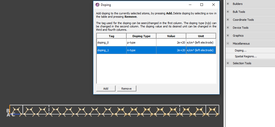
The 7.6 nm silicon device should consist of 28 Si layers (76.0284 Å) and 10.8612 Å left and right electrodes. The p and n doping levels should be both 2*1020 e/cm3 for this quite short Si device in order to get a reasonable electronic structure with fairly flat band edges near the electrodes and a small gap from the VBM and CBM to the Fermi level.
If you need more information on how to build a junction, please see the tutorial Silicon p-n junction.
NEGF calculation
The supplied script silicon_pn_junction.py uses a NEGF calculator with the settings given below.
Basis set: PseudoDojo and Low.
Exchange-correlation: GGA-1/2 and PBE.
k-point sampling: 4 Å density in the A and B directions.
Density mesh cutoff: 30 Ha.
Default output file:
silicon_pn_junction.hdf5.
Run the script using the Job manager (click the  button to start the calculation).
Photocurrent
You are now ready to calculate the photocurrent. Open the  Script Generator
and add a
Script Generator
and add a  Analysis from File.
Select the file
silicon_pn_junction.hdf5.Make sure the DeviceConfiguration object is ticked.
Next, in order to calculate the photocurrent, add the  block. Set the photon energy range to 0 – 5 eV with 31 points,
and set the k-point sampling to 9 x 9. Keep all other parameters at default values. You can also download the script
block. Set the photon energy range to 0 – 5 eV with 31 points,
and set the k-point sampling to 9 x 9. Keep all other parameters at default values. You can also download the script photocurrent.py. Send the script to the Job manager, save it as photocurrent.py, and click on the button to run the calculation.
Note
The photocurrent calculation takes ca. 3.5 hours with 4 MPI processes, so you may consider running the calculation on a remote computing cluster, if possible.
Once the calculation is done, you can see the file photocurrent.hdf5 in the LabFloor. Note that the calculation can be made faster by decreasing the number of photon energies and increasing the energy_resolution, leading to fewer electron energy points.
Select the Photocurrent_0 object of photocurrent.hdf5 on the LabFloor. Open the Photocurrent Analyzer in the right-hand panel.
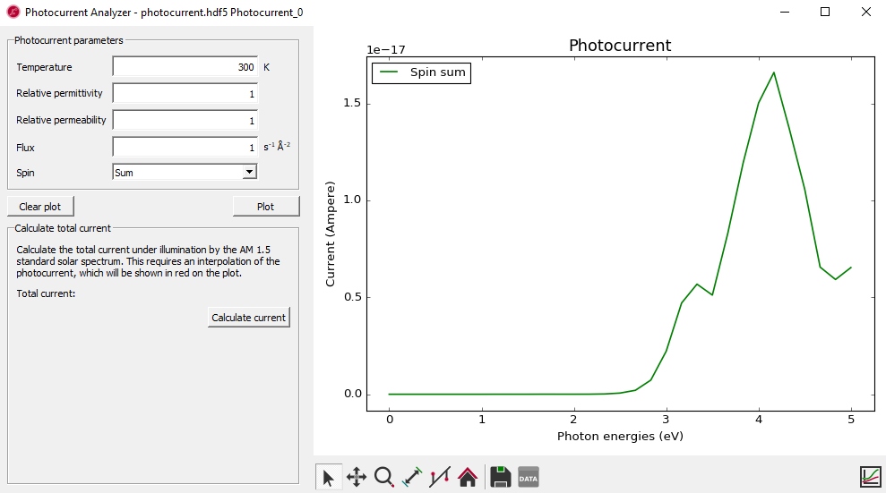
You can easily plot the current vs. photon energies by clicking Plot. This is shown in the figure below.
You can also calculate the total current based on illumination by the AM1.5 standard solar spectrum obtained from Solar spectra website. Once you click Calculate current, the interpolated photocurrent will be indicated by a red line. This interpolated function is multiplied with the flux from the reference spectrum at each photon energy, and the result is then numerically integrated to calculate the total current from the device under the given illumination.
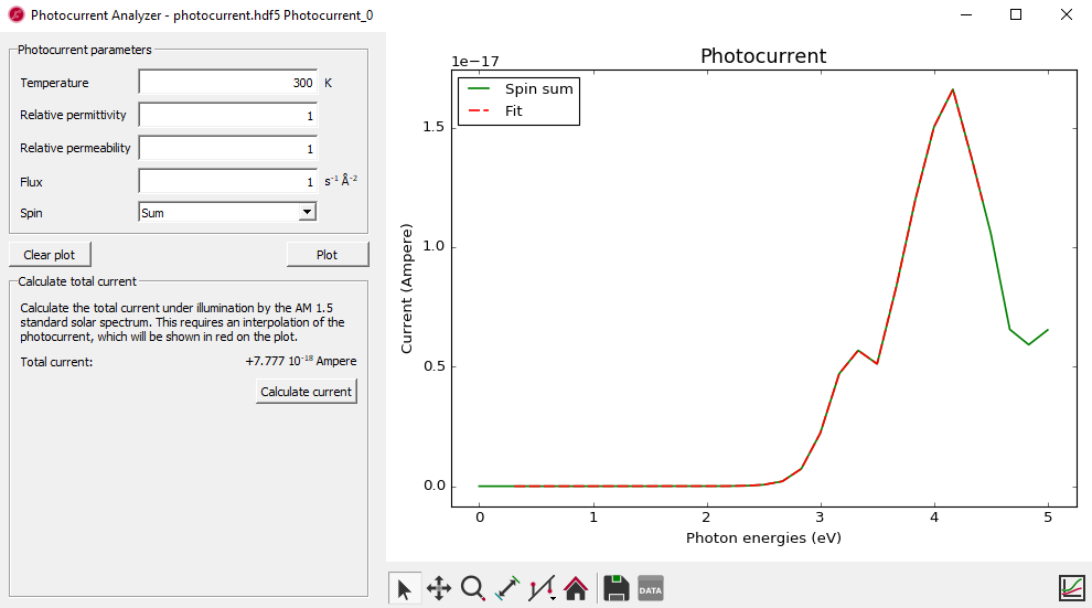
Fig. 82 The total current is calcuated as 7.777\(\cdot\)10-18 Ampere under the illumination by the AM 1.5 standard solar spectrum.
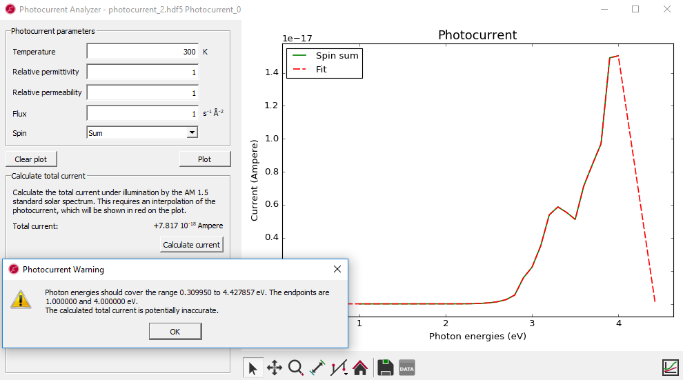
If the photon energies used to calculate the photocurrent do not cover the range of photon energies in the AM1.5 spectrumn, you will see a warning message. In this case, the interpolation will include data outside the data range, so the calculated total current may therefore be inaccurate. We therefore recommend to calculate the total current only from photocurrents covering the full range of the AM1.5 standard solar spectrum, which is 0.3 eV to 4.43 eV. Photocurrents covering a larger range is not a problem, as data outside the range of the reference spectrum simply do not contribute. The figure below shows an example of this.