Phonon-limited mobility in graphene using the Boltzmann transport equation
Version: Q-2019.12-SP1
In this tutorial you will learn how to calculate the phonon-limited mobility in graphene. The mobility will be calculated using the Boltzmann transport equation (BTE) with the electronic structure, phonons and electron-phonon coupling calculated using density functional theory (DFT).
The mobility \(\mu\) will be calculated using two different methods to calculate the relaxation times \(\tau\) entering the BTE:
Full angular (k,q)-dependence: in this method, the full dependency of \(\tau\) on the electron and phonon wave vectors \(\mathbf{k}\) and \(\mathbf{q}\) is taken into account, so that \(\tau = \tau(\mathbf{k},\mathbf{q})\). In the following, we will refer to this as the (k,q)-dependent method.
Isotropic scattering rate: in this method, only the energy dependence of \(\tau\) is considered, so that \(\tau = \tau(E)\), and \(\tau(E)\) is assumed to vary isotropically in momentum-space. In the following, we will refer to this as the E-dependent method.
As it will be shown, the two methods give essentially the same results, but the second method is considerably faster than the first one.
In the theory section, you can read about the theoretical background. A more comprehensive description can also be found in the paper [1].

Geometry and electronic structure of graphene
In the  Builder, add a graphene configuration by clicking
and searching for ‘Graphene’ in the structure database.
Builder, add a graphene configuration by clicking
and searching for ‘Graphene’ in the structure database.
Next, you have to increase the vacuum gap above and below the graphene. Click on and set the lattice parameter along the C-direction to C = 20 Å.
Center the configuration by clicking on , and press Apply.
Now click on the
 button to send the structure to the
  Script Generator. In the main panel of the Script Generator, set the Results file to
Graphene_relax.hdf5,
To perform an accurate calculation of the relaxation times \(\tau\) and the mobility \(\mu\), the first important step is to optimize the lattice parameters A and B and calculate the electronic band structure. In order to do this, add an LCAOCalculator block and in the Main section set the following parameters:

Set the Exchange correlation to LDA
Set the Pseudopotential to FHI
Set the Occupation method to Methfessel-Paxton
Set the Density mesh cutoff to 90 Ha
Set the k-point sampling to:
\(\mathrm{k_A}\) = 33
\(\mathrm{k_B}\) = 33
\(\mathrm{k_C}\) = 1
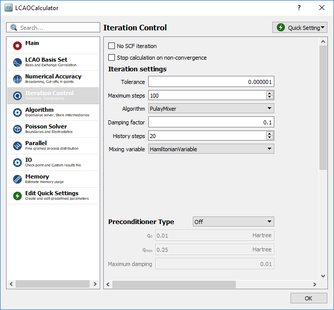
On the Iteration Control tab, Set the Tolerance to 0.000001, i.e. 10-6


Set the Force tolerance to 0.001 eV/Å
Untick Fix lattice vectors in the \(x\) and \(y\) directions.


Set the number of Points per segment to 100
Set the Brillouin zone route to G, K, M, G
Now, send the script to the  Job manager, save it as
 Graphene_relax.py, and click on the
 button to run the calculation.
When the calculation is done, click on the Bandstructure object contained
in the file Graphene_relax.hdf5 on the LabFloor and use the Bandstructure Analyzer to visualize the
band structure.

By placing the mouse cursor on top of a band, information about the band is shown. You see that the valence band (highlighted in yellow in the figure above) is number 3 and the conduction band is number 4. These are the two electronic bands relevant for the calculation of the mobility, and in the following we will concentrate on these two bands.
Phonons in Graphene
The next step is to calculate the dynamical matrix of graphene. In order to test the quality of the result you will also calculate the phonon band structure, which is based on the calculated dynamical matrix.
Open the Script generator , and create a new script:
Add an
 block and select BulkConfiguration_1 in
 Graphene_relax.hdf5.Add a

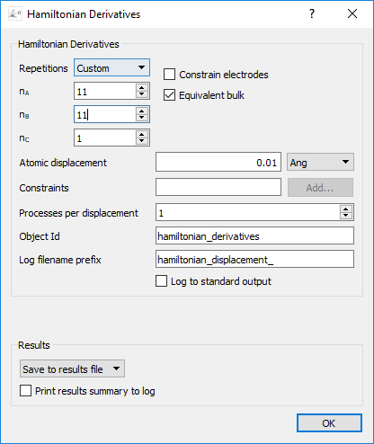
 block and modify the following settings:
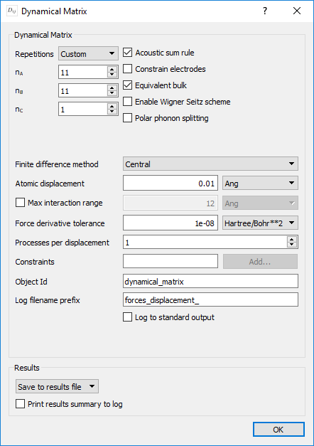
Set Repetitions to Custom
Set the Number of repetitions to:
\(\mathrm{n_A}\) = 11
\(\mathrm{n_B}\) = 11
\(\mathrm{n_C}\) = 1
Note
In previous versions of QuantumATK it was necessary to manually scale down the number of k-points when doing a DynamicalMatrix or HamiltonianDerivatives calculation to take into account the repeated cell. From QuantumATK-2019.03 and later versions the k-points are automatically scaled to maintain the same accuracy as the unit cell, and we can simply re-use the calculator settings.
Tip
Due to the large dimensions of the \(11 \times 11\) graphene super cell (242 atoms), the calculation of the DynamicalMatrix object is rather time consuming. However, the calculation can be parallelized over the atomic displacements. Since there are two atoms in the graphene unit cell, and each is displaced in the \(x\), \(y\) and \(z\) directions, there are in total 6 calculations to be performed. Maximum efficiency is obtained when the number of calculations times the value of the parameter Processes per displacement matches the total number of cores used for the calculations. In the present case, the calculation takes about 30 minutes if Processes per displacement = 4 and the calculation is run on 24 cores.
Add an
 block and set the following parameters:
Set the number of Points per segment to 100
Set the Brillouin zone route to G, M, K, G
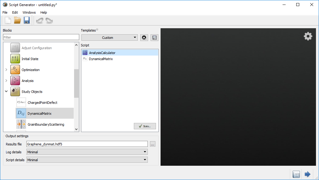
Finally, in the main panel of the Script Generator set the Default output file to
Graphene_dynmat.hdf5, send the script to the
Job manager, save it as Graphene_dynmat.py and click on the button to run the calculation.
Warning
Remember to make the file Graphene_relax.hdf5 available for the script if you are running on a cluster. In the Job Manager you can use the I/O tab to transfer additional files together with a script. In this case, you may also need to modify the path in the script before submitting to the cluster, to make sure it points at the correct location of the file.
When the calculation is done, go back to the in the LabFloor, and inspect the
PhononBandstructure object contained in the file Graphene_dynmat.hdf5 using Compare data or
PhononBandstructure Analyzer. The calculated phonon band structure should match with that shown in the figure
below.

Fig. 28 Phonon bandstructure. There are three acoustic modes: The lowest, out-of-plane mode (ZA) has a \(\propto \mathbf{q}^2\) for small \(\mathbf{q}\), while the two next have linear \(\mathbf{q}\)-dependence with a constant velocity for small \(\mathbf{q}\). The transverse acoustic (TA) mode is lower in energy than the longitudinal acoustic (LA) mode.
Mobility of graphene
In the following, the procedure to calculate the electron mobility in graphene will be described. Provided that one has already calculated the electronic structure and dynamical matrix of the system, the following three steps are necessary to evaluate the mobility:
Calculation of the Hamiltonian derivatives
Calculation of the Electron-phonon couplings
Calculation of the Mobility
The two methods to calculate \(\mu\) described above differ in the way in which steps 2 and 3 are carried out. These two steps will therefore be described separately for each method. The procedure for the (k, q)-dependent method is outlined in sections 1, 2A and 3A, whereas the procedure for the energy-dependent method is outlined in in sections 1, 2B and 3B
1. Hamiltonian derivatives
In order to calculate the electron-phonon coupling matrix, it is necessary to calculate the derivative of the Hamiltonian \(\partial \hat{H}/\partial R_{i,\alpha}\) with respect to the coordinate of the \(i\)-th atom along the Cartesian direction \(\alpha\).
Open the Script generator , and modify the script as follows:
Add an
block and select BulkConfiguration_1 in Graphene_relax.hdf5.Add a
 block and set the Number of repetitions to:
\(\mathrm{n_A}\) = 11
\(\mathrm{n_B}\) = 11
\(\mathrm{n_C}\) = 1
Warning
It is important that the number of repetitions matches the calculation of the dynamical matrix.
In the main panel of the Script Generator, set the Results file to
Graphene_dHdR.hdf5, send the script to the Job manager, save it as
Graphene_dHdR.py and click on the button to run the calculation.
Note
As for the DynamicalMatrix, the calculation of the HamiltonianDerivatives is rather time consuming, but can be parallelized over the atomic displacements. In the present case, the calculation takes around 1 hour if it is run on 24 cores with Processes per displacement = 4 .
2A. Electron-Phonon couplings: (k,q)-dependent method
In order to calculate the lifetimes \(\tau(\mathbf{k},\mathbf{q})\) and the mobility \(\mu\), we need to calculate the electron-phonon coupling matrix on a fine grid of \(\mathbf{k}\)- and \(\mathbf{q}\)-points.
Open the Script generator , and modify the script as follows:
Add an
block and select BulkConfiguration_1 in Graphene_relax.hdf5.Add an
 block.
You will notice that two additional blocks have been also added:
In the present case, both the dynamical matrix and the Hamiltonian derivatives have been calculated already and can be
re-used. As they are study objects, this is automatically detected by QuantumATK if the provided filename and other input parameters are the same. Open each of them and change the repetitions to 11x11x1 and the filenames to Graphene_dynmat.hdf5 and Graphene_dHdR.hdf5, respectively.
Now set the parameters in the block as
shown below. We will sample k-points in a small area around the \(\mathrm{K}\)-point at [1/3, 1/3, 0], and q-points in a small area around the \(\mathrm{\Gamma}\)-point at [0,0,0].
Tip
If you are unsure of the coordinates of a particular symmetry point you may use the built-in functionality of the BravaisLattice class, f.ex. like this:
k0=bulk_configuration.bravaisLattice().symmetryPoints()['K'])
Warning
For production calculations, it is strongly recommended to always converge the sampling resolution in q- and k-space. The above settings are a result of such a study, with more information shown in the appendix: Convergence of q- and k-point sampling
In the main panel of the Script Generator, set the Results file to
Graphene_eph.hdf5. Send the script to the Job manager, save it as
Graphene_eph.py and click on the button to run the calculation.
Warning
For graphene, we need quite dense samplings in \(\mathbf{k}\)- and \(\mathbf{q}\)-space, and therefore we have chosen to sample very finely a small area around the relevant high-symmetry points. This still includes the full angular dependence, but neglects inter-valley scattering. We therefore recommend to sample the entire Brillouin zone if this could be an important effect.
Note
Sampling the \(\mathbf{k}\)- and \(\mathbf{q}\)-space using dense meshes means that the calculation might become very time consuming. Contemporary versions of QuantumATK automatically detect the relevant regions of \(\mathbf{k}\)- and \(\mathbf{q}\)-space, and do not compute matrix elements which will not contribute, considerably decreasing the computational time and memory requirements. The two parameters energy_tolerance and initial_state_energy_range govern the filters which reduce the number of calculated coupling elements. More information about these two parameters can be found on the manual page: ElectronPhononCoupling.
As QuantumATK parallelizes over \(\mathbf{k}\)- and \(\mathbf{q}\)-points, a high number of MPI processes can be used if sufficient memory is available. In the present case, the calculation took approximately 10 hours on a 16-core node on a cluster.
3A. Mobility: (k,q)-dependent method
Now open a new Script Generator window and add an block and then a  block. In the block, select the file
 Graphene_relax.hdf5 and load BulkConfiguration_1 included in the file. Remove the , and blocks, and replace them with a  block. This allows us to easily add arbitrary code to any script without editing the full script manually. Open the block, and write the following:
electron_phonon_coupling = nlread('Graphene_eph.hdf5', ElectronPhononCoupling)[0]
Set the parameters for the block as shown below:
Leave the Method at Full angular (k,q)-dependence
Set the Fermi shift to 0.13 eV
Untick Calculate Hall coefficients
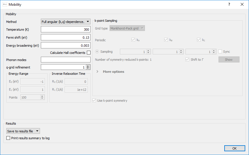
Note
The Fermi shift of 0.13 eV corresponds to a carrier concentration of \(n = 10^{12} \mathrm{cm^{-2}}\)
In the main panel of the Script Generator, set the Results file to
Graphene_mu-full.hdf5, send the script to the Job manager, save it as
Graphene_mu-full.py and click on the button to run the calculation. It should take no more than a few minutes on a laptop.
Note
You will get a notification that the Mobility block is invalid. You can ignore this warning, as NanoLab does not parse the Code snippet block and is thus unaware of the ElectronPhononCoupling object that will be loaded there.
Once the calculation is done, select the file Graphene_mu-full.hdf5, and on the LabFloor, select the
Mobility object, and click on Text Representation. You should now see the following:
 +------------------------------------------------------------------------------+
 | Mobility Report                                                              |
 | ---------------------------------------------------------------------------- |
 | Input parameters:                                                            |
 |     Temperature       = 300.00 K                                             |
 |     Fermi level shift = 0.13 eV                                              |
 |     Energy broadening = 0.0030 eV                                            |
 |     q-grid refinement = 1                                                    |
 |                                                                              |
 +------------------------------------------------------------------------------+
 | Trace of linear responce tensors:                                            |
 +------------------------------------------------------------------------------+
 |                                                                              |
 | Electrons:                                                                   |
 |                                                                              |
 |     Mobility                 =  2.34e+05 cm^2/(V*s)                          |
 |     Conductivity             =  4.19e+01 S/m                                 |
 |     Seebeck coefficient      = -1.94e-05 V/K                                 |
 |     Thermal conductivity     =  2.43e-04 W/(m*K)                             |
 |     Carrier density (2D, xy) =  2.24e+06 cm^-2                               |
 |                                                                              |
 |                                                                              |
 | Holes:                                                                       |
 |                                                                              |
 |     Mobility                 =  8.66e-04 cm^2/(V*s)                          |
 |     Conductivity             =  1.19e-01 S/m                                 |
 |     Seebeck coefficient      =  1.14e-03 V/K                                 |
 |     Thermal conductivity     =  1.18e-05 W/(m*K)                             |
 |     Carrier density (2D, xy) =  1.72e+12 cm^-2                               |
 |                                                                              |
 +------------------------------------------------------------------------------+
The calculated electron mobility, highlighted in yellow, is \(2.34 \cdot 10^{5}\ \mathrm{cm^{2} V^{-1} s^{-1}}\), and agrees well with previously reported data at room temperature and \(n = 10^{12} \mathrm{cm^{-2}}\) [2].
Note
Note that the carrier density listed here is significantly lower than \(n = 10^{12} \mathrm{cm^{-2}}\). The carrier density is calculated independently from the mobility, and converges much more slowly than the mobility itself. In this tutorial, the focus is on achieving a converged value for the mobility - converging also the carrier density would require inclusion of more \(\mathbf{k}\)-points and/or a larger region in \(\mathbf{k}\)-space in the ElectronPhononCoupling calculation.
Alternatively, you can calculate the carrier density with a finer sampling directly from the DensityOfStates object: carrier_density_test.py.
Tip
Starting from version Q-2019.12, QuantumATK NanoLab includes a Mobility Analyzer. This will be presented in a future update of this tutorial.
2B. Electron-Phonon couplings: energy-dependent method
We will now calculate the electron-phonon couplings to be used for the calculation of the energy-dependent relaxation times \(\tau(E)\). We will assume that the relaxation times vary isotropically in \(\mathbf{k}\)-space. This means that it will be sufficient to evaluate the electron-phonon coupling matrix for a number of \(\mathbf{k}\)-points along a line through one of the Dirac (K) points, thereby reducing significantly the computational workload of the calculation.
Open the Script generator , and modify the script as follows:
Add an
block and select BulkConfiguration_1 in Graphene_relax.hdf5.Add an
block.
You will notice that two additional blocks have been also added:
In the present case, both the dynamical matrix and the Hamiltonian derivatives have been already calculated and can be
re-used. As they are study objects, this is automatically detected by QuantumATK if the provided filename and other input parameters are the same. Open each of them and change the repetitions to 11x11x1 and the filenames to Graphene_dynmat.hdf5 and Graphene_dHdR.hdf5, respectively.
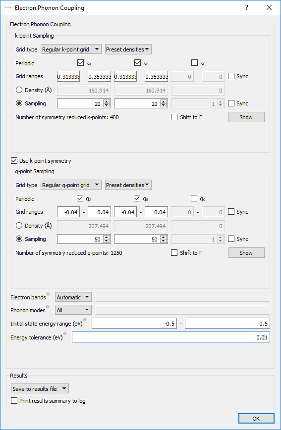
In the block, modify the parameters as follows:
In the k-point sampling, set the Grid type to Regular k-point grid, and the sampling parameters as shown in the figure below.
Note
As you can see from the figure, the \(\mathbf{k}\)-space is sampled only along a line!
In the q-point sampling, set the Grid type to Regular q-point grid, and the sampling parameters as shown in the figure below.
Set the Energy tolerance to 0.01 (eV) and the Initial state energy range to go from -0.5 to 0.5.

In the main panel of the Script Generator, set the Results file to
Graphene_eph-line.hdf5, send the script to the Job manager, save it as Graphene_eph-line.py
and click on the button to run the calculation.
Note
Since here we sample the \(\mathbf{k}\)-space only along a line, the calculation will in general be faster than the one described in section 2A. In the present case, the calculation took approximately 50 minutes on a 16-core node on a cluster, or about 1/10th of the full calculation in section 2A.
3B. Electron mobility: energy-dependent method
We will now use a two-step procedure to evaluate the room-temperature mobility \(\mu\) based on the energy-dependent relaxation times \(\tau(E)\):
In the first step, the \(\mathbf{k}\)- and \(\mathbf{q}\)-dependent relaxation times \(\tau(\mathbf{k},\mathbf{q})\) are evaluated along the line outward from the K-point.
In the second step, the values of \(\tau(\mathbf{k},\mathbf{q})\) are averaged in \(\mathbf{k}\)-space to obtain the values of \(\tau(E)\), which are then used to calculate the mobility \(\mu\).
Now open a new Script Generator window and add an block and then a block. In the block, select the file Graphene_relax.hdf5 and load BulkConfiguration_1 included in the file. Remove the and objects and replace the with a block. Open the block, and write the following:
electron_phonon_coupling = nlread('Graphene_eph-line.hdf5', ElectronPhononCoupling)[0]
Finally, set the parameters in the block as shown below:
-
Set the Method to Full angular (k,q)-dependence
Set the Fermi shift to 0.13 eV
Untick Calculate Hall coefficients

Note
Note that we choose a \(\mathbf{k}\)-line direction somewhat arbitrarily here. The point is that a low number of \(\mathbf{k}\)-points can be used to generate an energy dependent rate. An alternative to a line could be to coarsely sample the entire BZ to capture the anisotropy in \(\mathbf{k}\)-space, but with fewer points than needed in the full (\(\mathbf{k}\), \(\mathbf{q}\))-dependent method.
In the main panel of the Script Generator, set the Results file to
Graphene_mu-line-full.hdf5, send the script to the Job manager,save it as
Graphene_mu-line-full.py and click on the button to run the calculation. You will again see a warning that the script might be invalid, and you should ignore it this time as well.
Once the calculation is done, you are ready to calculate the mobility using the isotropic scattering rate method.
In this case, you will re-use the bulk configuration and the full angular (\(\mathbf{k}\), \(\mathbf{q}\)) -dependent mobility from the
Graphene_relax.hdf5 and Graphene_mu-line-full.hdf5 files.
Go back to the Script generator, and open the block before the Mobility icon . Change the contents to:
mobility_full = nlread('Graphene_mu-line-full.hdf5', Mobility)[0]
Then modify the block as follows:
-
Set the Method to Isotropic scattering rate
Set the Fermi shift to 0.13 eV
Untick Calculate Hall coefficients
Set the following values of the Energy Range:
\(\mathrm{E_0}\) = -0.24 eV
\(\mathrm{E_0}\) = 0.24 eV
Points = 100
Set the k-point Sampling to \(99 \times 99 \times 1\)

In the main panel of the Script Generator, set the Results file to
Graphene_mu-line-iso.hdf5. Send the script to the Editor, change mobility_object=None, to mobility_object=mobility_full, and remove this line:
inverse_relaxation_time=numpy.linspace(0, 1e+12, 100)*Second**-1,
Send it to the Job manager, save it as Graphene_mu-line-iso.py and click on
the button to run the calculation. This should take no more than a minute on a modern laptop.
Once the calculation is done, open the file Graphene_mu-line-iso.hdf5, select the
Mobility object in the LabFloor and click on Text Representation.
 +------------------------------------------------------------------------------+
 | Mobility Report                                                              |
 | ---------------------------------------------------------------------------- |
 | Input parameters:                                                            |
 |     Temperature       = 300.00 K                                             |
 |     Fermi level shift = 0.13 eV                                              |
 |     Energy broadening = 0.0030 eV                                            |
 |     q-grid refinement = 1                                                    |
 |                                                                              |
 +------------------------------------------------------------------------------+
 | Trace of linear responce tensors:                                            |
 +------------------------------------------------------------------------------+
 |                                                                              |
 | Electrons:                                                                   |
 |                                                                              |
 |     Mobility                 =  2.53e+05 cm^2/(V*s)                          |
 |     Conductivity             =  1.73e+07 S/m                                 |
 |     Seebeck coefficient      = -3.00e-05 V/K                                 |
 |     Thermal conductivity     =  9.31e+01 W/(m*K)                             |
 |     Carrier density (2D, xy) =  8.55e+11 cm^-2                               |
 |                                                                              |
 |                                                                              |
 | Holes:                                                                       |
 |                                                                              |
 |     Mobility                 =  1.89e+06 cm^2/(V*s)                          |
 |     Conductivity             =  5.72e+04 S/m                                 |
 |     Seebeck coefficient      =  1.14e-03 V/K                                 |
 |     Thermal conductivity     =  5.74e+00 W/(m*K)                             |
 |     Carrier density (2D, xy) =  3.78e+08 cm^-2                               |
 |                                                                              |
 +------------------------------------------------------------------------------+
The calculated value for the electron mobility, highlighted in yellow above, is \(2.53 \cdot 10^{5}\ \mathrm{cm^{2} V^{-1} s^{-1}}\), in good agreement with the value obtained by using the full (\(\mathbf{k}\), \(\mathbf{q}\)) -dependent method.
Temperature dependence of the mobility: (k,q)-dependent method vs. energy-dependent method
A more stringent test for the reliability of the energy-dependent method is to calculate the temperature dependence of the mobility in an energy range up to room temperature.
In the (k,q)-dependent method, this can be done by simply modifying the value of the target temperature in the
Mobility analysis object. temperature_dependence_full_mobility.pyIn the energy-dependent method, the two-step procedure must be repeated for each temperature, and the target temperature has to be set both when calculating the values of the \(\mathbf{k}\)- and \(\mathbf{q}\)-dependent relaxation times \(\tau(\mathbf{k},\mathbf{q})\) along the line, and when calculating the energy-dependent relaxation times \(\tau(E)\).
temperature_dependence_isotropic_mobility.py
As it can be seen from the figure below, where the \(T\)-dependency of \(\mu\) is calculated in the
temperature range \(100 \mathrm{K} \leq T \leq 300 \mathrm{K}\), both methods reproduce well the expected
\(1/T\) behavior of \(\mu\). Script to create the plot: plot_temperature_dependence_mobility.py

Convergence of q- and k-point sampling
In order to select the appropriate samplings in \(\mathbf{k}\)- and \(\mathbf{q}\)-space, we first studied the mobility as a function of the number of \(\mathbf{q}\)-points, for a fixed sampling of \(\mathbf{k}\)-points:

We see that the mobility is reasonably converged for 50 \(\mathbf{q}\)-points and above. This corresponds to a density of at least 200 \(Å\). We then study the mobility as a function of \(\mathbf{k}\)-points, and see that it converges very quickly in this case. We chose to use 20 k-points, corresponding to a density of about 160 \(Å\).

Warning
This convergence study is only valid for this combination of system and computational settings. You should always study convergence for your system of interest and chosen computational model.
Theory section
The mobility \(\mu\) is related to the conductivity \(\sigma\) via
where \(n\) is the carrier density, \(e\) is the electronic charge.
In this tutorial, you will calculate the conductivity using the semi-classical Boltzmann transport equation (BTE). In the case of zero magnetic field and a time-independent electric fields in the steady state limit the BTE simplifies to:
The right hand side (RHS), often called the collision integral, describes different sources of scattering and dissipation that drives the system towards steady state. The left hand-side is approximated to linear order in the electric field by changing to the equilibrium distribution.
The electron-phonon scattering is described by the collision integral. Most commonly this is approximated by a relaxation time:
describing quasielastic scattering on acoustic phonons (relaxation time approximation). We let \(\lambda\) label the phonon modes, \(n\) the electronic bands, \(\mathbf{k}\) the electron momentum. The transition rate from a state \(|\mathbf{k}n\rangle\) to \(|\mathbf{k}'n'\rangle\) is obtained from Fermi’s golden rule (FGR):
\[\begin{split}P_{\mathbf{k}\mathbf{k'}}^{\lambda nn'} &= \frac{2\pi}{\hbar} |g_{\mathbf{k}\mathbf{k'}}^{\lambda n n'}|^2 [ n_{\mathbf{q}}^{\lambda} \delta \left(\epsilon_{\mathbf{k}'n'}-\epsilon_{\mathbf{k}n}-\hbar \omega_{q \lambda} \right) \delta_{\mathbf{k}',\mathbf{k}+\mathbf{q}} \\[.5cm] &+ (n_{\mathbf{-q}}^{\lambda}+1) \delta \left( \epsilon_{\mathbf{k}'n'}-\epsilon_{\mathbf{k} n}+\hbar \omega_{-q \lambda} \right) \delta_{\mathbf{k}',\mathbf{k}-\mathbf{q}} ],\end{split}\]
where the first and last terms in the square brackets describes phonon absorption and emission, respectively. The electron-phonon coupling matrix elements \(|g_{\mathbf{k}\mathbf{k'}}^{\lambda n n'}|\) are in ATK calculated using the ElectronPhononCoupling analysis module.
The general electron-phonon collision integral is given by
Relaxation time approximation
In the relaxation-time approximation (RTA) one assumes a special simplified form of the RHS/collision integral:
where \(\delta f_{\mathbf{k}n} = f_{\mathbf{k}n}-f^0_{\mathbf{k}n}\). The linearized BTE becomes:
Hereby we find the solution:
The relaxation-time can be evaluated from the general collision integral, (10). However, the specific form in eqn. (11) only applies in the limit of quasielastic scattering (\(\omega_{q \lambda}\rightarrow 0\)), in which case the collision integral, in eqn. (10), simplifies significantly:
since \(P_{\mathbf{k}\mathbf{k'}}^{nn'} = P_{\mathbf{k}'\mathbf{k}}^{n'n}\) in this limit.
We then obtain the expression for the scattering rate or inverse relaxation-time:
where we applied the detailed balance equation in this limit, \(P_{\mathbf{k}\mathbf{k'}}^{nn'}(f^0_{\mathbf{k}'n'}-f^0_{\mathbf{k}n})=0\), and assumed isotropic scattering.
To evaluate the relaxation time we introduce the scattering angle
where \(\mathbf{v}_{\mathbf{k}n}\) is the electron velocity. Following [1] we obtain
Mobility
Once knowing the relaxation times one obtain the mobility as:
where the factor 2 accounts for spin degeneracy.