Calculating Reaction Rates using Harmonic Transition State Theory
Introduction
In this tutorial, you will learn to use QuantumATK for calculating reaction rates using the nudged elastic band (NEB) method and harmonic transition state theory (HTST). These two techniques are a powerful combination that allow researchers to model solid-state reactions (or more generally any rare event dynamics). Typically, reactions in the solid state are too slow to efficiently study with molecular dynamics (MD) simulations. HTST, on the other hand, takes a statistical mechanics approach to computing the reaction rate. Therefore, in constrast to MD simulations, the amount of computational work required to calculate a reaction rate is independent of the timescale of the reaction.
Theory
HTST [1] is derived from a more general formalism known as transition state theory (TST) [2][3]. TST works by defining a transition state (a hyperplane) that separates the reactant from the products. Then the reaction rate is calculated as the probability of finding the system at the transition state relative to the entire reactant state, multiplied with the rate of crossing from the reactant region to the product region at the transition state. In general, TST is difficult to use, because it requires a definition of the transition state hyperplane. Additionally, calculating the probability of being at the transition state requires evaluating the full partition function of the transition state region and the reactant region, which is computationally prohibitive when using density functional theory, and challenging even for fast classical potentials.
TST can be made a more practically useful theory by making two simplifying assumptions. The first is that saddle points on the potential energy surface represent “bottle neck” regions that separate reactant from product configurations. This solves the issue of determining the hyperplane in TST by defining it as the hyperplane normal to the unstable direction at the saddle point. The second is that the potential energy surfaces around the reactant configuration and the saddle point are locally harmonic (quadratic). This allows for a second order Taylor series expansion of the potential energy surface at those points and the resulting configuration integrals needed in TST are now closed-form expressions. The combination of these two assumptions is called HTST.
HTST is a good approximation for many solid-state reactions, because the energy barriers are often large compared to the average kinetic energy in the system (\(k_{\rm B} T\)). This is important because it ensures that the system reaches a local equilibrium between reactive events. If the barriers are relatively small compared to the thermal energy, then there are dynamical correlations in the trajectory. This means that the history of the trajectory is an important factor in determining the reaction rate and would require the use of a more sophisticated statistical model. Another reason that solid-state reactions are described well by HTST is that the harmonic approximation is often valid. Near the saddle points the potential energy rises rapidly and creates a small bottleneck region, however, in some “soft” systems (e.g. conformation changes in a protein) the potential energy is relatively flat in the region around the saddle point and is not well characterized by harmonic expansion of the saddle point.
The first step in using HTST is to find the saddle point associated with the reaction in question. There are a number of techniques that can be used, but here we will use the NEB. NEB optimization can be performed in such a way that one of the images converges to a saddle point (as opposed to all the images being evenly spaced along the reaction coordinate). This is called climbing image NEB (CI-NEB) and an optimized CI-NEB should have a saddle point as its highest energy image.
Once the saddle point has been obtained the following formula is used to calculate the reaction rates:
where \(N\) is the number of atoms; \(\nu^{\rm R}_i\) and \(\nu^{\rm S}_i\) are the stable (real valued) normal mode frequencies at the reactant and saddle point (the \(3N-1\) at the saddle is due to there being exactly one imaginary frequency at the saddle); \(E^{\rm R}\) and \(E^{\rm S}\) are the energies at the minimum and saddle point; \(k_{\rm B}\) is Boltzmann’s constant; and \(T\) is the temperature.
The functional form of HTST is analogous to the empirically derived Arrhenius rate law:
The pre-exponential factor, \(A\), in the Arrhenius rate law corresponds to the ratio of the product of the vibrational modes at the minimum over the product of the stable vibrational modes at the saddle in HTST. This can be interpreted as an “attempt frequency”, i.e. the number of times per second that the system vibrates along the reaction direction.
The activation energy, \(E_{\rm a}\), in the Arrhenius rate law is defined as the difference in energy between the saddle and minimum in HTST. The exponential term represents the Boltzmann probability that a vibrational along the reaction direction will overcome the barrier and continue into the product state.
Thus, the HTST rate equation can be interpreted as:
Note
In most systems, the prefactor does not change significantly (ca. a factor of 10) from reaction to reaction. However, the exponential term (the Boltzmann probability of the system being at the transition state) can easily span 10 orders of magnitude. This is because most solid-state reactions are thermally activiated processes, whose rate primary depends upon the energy barrier.
Despite the small contribution of the prefactor to the difference in rate between different mechanisms it can be more computationally expensive to compute than the energy barrier.
It is thus recommended to experiment with the system to see if it is neccessary to compute the prefactor every time. In reactions involving light atoms (first two rows of the period table) the prefactor is often in the order of 1014 Hz, while for heavier metal atoms it may be as small as 1011 Hz. These frequencies are related to a typical vibrational period in these systems, which primarily depends on the atomic mass.
Modeling Pt Adatom Diffusion on Pt(100)
As an model system we will examine Pt adatom diffusion on a Pt(100) surface. There are at two well known mechanisms for adatom diffusion on this surface. The first is the “hop” mechanism where the adatom directly moves to an adjacent hollow site. The second is the “exchange” mechanism where the adatom exchanges places with a surface atom and displaces it into an adjacent hollow site.
There are several interesting things we will learn from this system. The first is that although DFT and classical potentials often agree about equilibrium properties, where the classical potentials have been fit, the agreement is often quite bad near saddle points. Often saddle points describe bond breaking and bond formation steps that can be particularly challenging to describe in many classical potentials, especially those potentials that make use of explicit angle terms as is often used to describe Si and C bonding. The second is that what may initially look like a simple one step reaction sometimes actually involves multiple steps. It is not uncommon to encounter a relatively unstable reaction intermediate between the chosen initial and final geometries. This will be an important point to understand since, formally, HTST only describes elementary single step reactions.
Constructing the Pt(100) surface
In the Builder click and then search for “platinum”. A list of structures containing platinum will appear, scroll through them to find “Platinum” and double click on it.
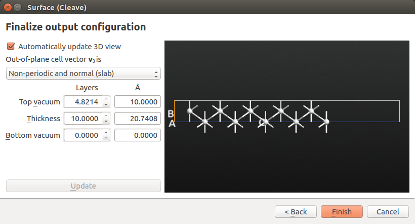
Then click and set the Miller indices to (100) and click Next. Create a 2x2 surface lattice and click Next. Then choose the Out-of-plane cell vector to be Non-periodic and normal (slab), set the thickness to 5 layers, and click Finish.
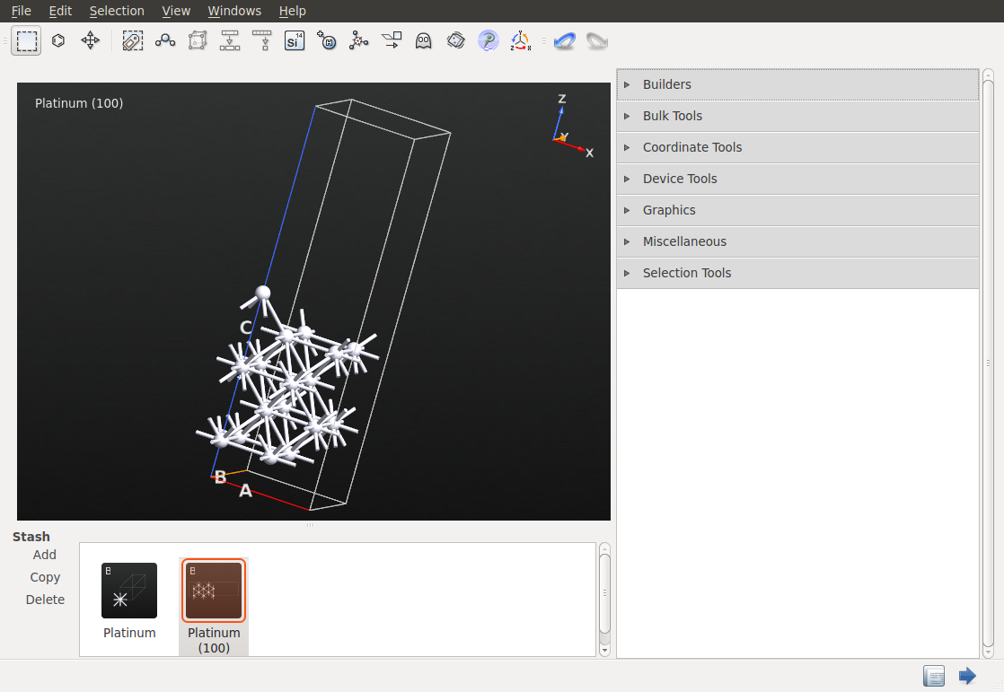
For later visualization it is nice to center the slab model in the x-y plane. To do this click , uncheck the C direction and click Apply.
Delete all but one of the atoms in the 5th layer. The remaining atom will be the diffusing adatom in the NEB calculation.
Constructing the NEB Configuration
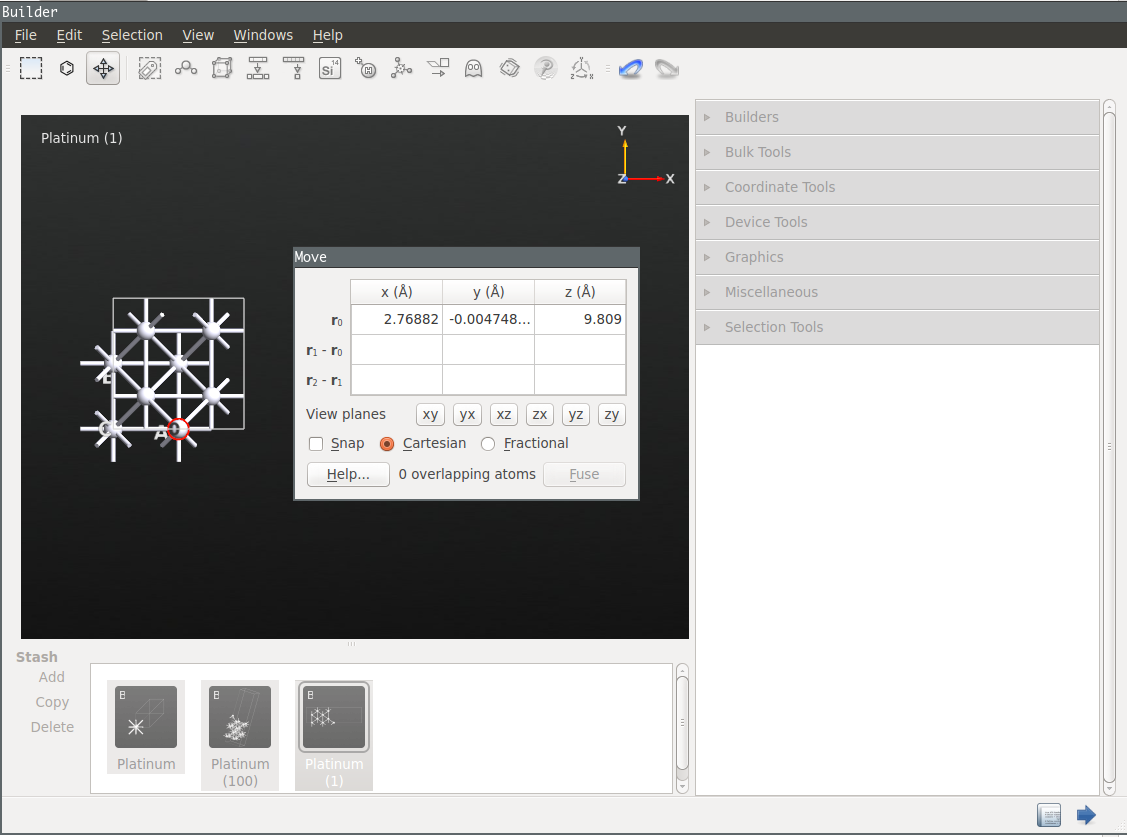
Make a copy of the configuration by clicking the Copy button in the Stash. Double click on the new configuration. Now select the adatom and click on the move tool in the toolbar and drag the adatom to and adjacent hollow site. This is easiest to do if you first camera view plane to the XY plane.
Click and drag both configurations from the stash to the initial and final drop zones. Click on Constraints and select the bottom most layer. Click Add tag from Selection, then change the constraint type from None to Fixed and click OK. Change the NEB method from Linear to Image Dependent Pair Potential. In this case, as few as 5 images should work well, since it is a relatively simple reaction coordinate. Set the Maximum distance to 1 Å and click Create.
Right click on the NEB configuration in the Stash and select .
Optimizing the NEB and Calculating the HTST Rate
Double click on New Calculator in the Blocks list to add a calculator to the Script. Now double click on the just added New Calculator in the Script. Change the k-point sampling to be 3x3x1 and the Exchange correlation function to GGA. Then click OK.
Double click on in the Blocks list and the double click on OptimizeGeometry in the Script list. Change the Force Tolerance to 0.01 eV/Å. Then click Add Constraints, select the bottom most layer of atoms, click Add tag from Selection, and change the constraint type from None to Fixed. Check the Climbing Image Method check box as well as Optimize end points.
It is crucial that a CI-NEB calculation is performed. If a regular NEB optimization is used then the images will be equally spaced along the reaction coordinate. This means that there will most likely not be an image at the saddle point. While, a converged CI-NEB calculation should have a saddle point as the highest energy image.
Note
In this tutorial, we are optimizing the NEB end points and the intermediate images in one step. This works fine for this simple case where the endpoints are close to their optimized geometries, however, it is typically a good idea to break this process up into three steps:
Optimize the initial end point.
Optimize the final end point.
Create the NEB configuration from the optimized endpoints and optimize it.
This approach allows you to analyze and verify the optimized end points to ensure that the geometry optmization did not significantly alter them.
Double click on in the Blocks list then double click on the HTSTEvent in the Script list. There are two options for determining the prefactor in the HTST rate equation (see the first equation in the introduction).
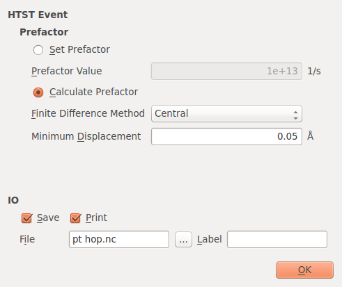
The first way to calculate the prefactor is to calculate the dynamical matrix for a subset of the atoms in the system. The atoms included in the calculation are those that move by by more than the Minimum Displacement parameter along the reaction coordinate along with their nearest neighbors (as determined using covalent radii). The second method is to simply set the prefactor to a known value.
Change the default output file pt hop.nc. Then either save the script and
run it with atkpython or send it to the Job Manager to run it.
The calculation may take a couple of hours depending upon your hardware and the number of MPI processes used.
Note
It is possible that the highest energy image of the converged CI-NEB calculation will not be a first order saddle point. This will be detected when the frequencies at the saddle point are calculated. An error message will be printed to the log and the calculated frequencies will be printed. There are a number of reasons why this may occur:
The NEB optimization did not converge. Consider increasing the maximum number of steps in the optimization and double checking the input geometries to be sure that the initial guess is reasonable.
The NEB optimization may have converged, but the force tolerance is too large. Try making the force tolerance smaller. A good value for many systems is \(10^{-2}\) eV/Å, but it may sometimes be required to use \(10^{-3}\) eV/Å.
If negative frequencies at the saddle still persist, then it is possible the NEB has converged to a second-order saddle point (i.e. a saddle point with two negative frequencies). In this case you should try to build a different initial guess for the NEB configuration to see if it will converge to the correct first-order saddle point.
Analyzing the Results
After the calculation finishes the file pt hop.nc should contain the initial
and converged NEB configurations, as well as the HTSTEvent. Click on the second
NEB configuration and click on the Movie Tool in the panel on the right.

The potential energy curve shows that the barrier is about 1.3 eV. The movie of the reaction visualizes the expected hopping process. There is a single barrier between the initial and final state. Close the Movie Tool window. Select the HTSTEvent object on the LabFloor and click the HTST Rates plugin in the panel on the right.
Information about about the reaction such as the barriers and prefactors are shown. The rate can be calculated at any temperature by changing the temperature value, which is 300 K by default.
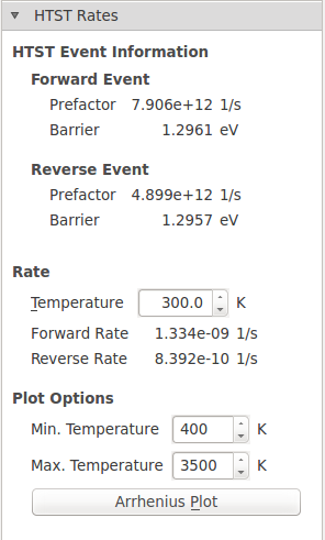
The forward and reverse barrier and prefactor should be identically theoretically, however, in practice they are not. This is due to small differences in the NEB endpoint geometries since each was minimized from a slightly different starting structure. Also, since this is an ATK-DFT calculation, translational symmetry is not perfectly preserved due to the eggbox effect. This effect describes the relationship between the real-space grids used to represent the charge density and potentials and the positions of the atoms. These grids will be aligned differently with different atoms thus breaking the translational symmetry. The effect is very small for the total energy in this case (< 1 meV), but is more pronounced for the prefactor, where it differs by a factor of 1.6. These errors can be minimized by increasing the Density mesh cut-off in the ATK-DFT calculator settings, but it increases the computational cost of the simulation and may not be necessary to get meaningful results.
It is also possible to make an Arrhenius plot to show the temperature dependence of the HTST rate. An Arrhenius plot is the \(\log({\rm rate})\) vs \(1/T\). When the temperature dependence is plotted this way, the plots will always be straight lines. The slope of the line is \(-\Delta E/k_{\rm B}\) and the y-intercept is the prefactor. From the plot it is easy to interpret that the prefactor is the maximum possible rate predicted by HTST.
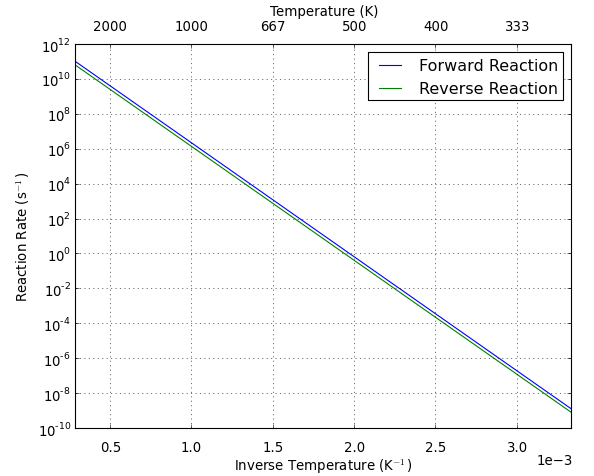
The reaction rate for Pt diffusion via the hopping mechanism is extremely slow at room temperature. The average time between reactions (the inverse of the rate) is on the order of centuries. However, at 600 K we can expect the reaction to occur tens of times per second.
Calculating the Rate for Multiple Elementary Reaction Steps
The exchange mechanism for Pt adatom diffusion on Pt(100) is an interesting case study, because it does not proceed via a single elementary reaction like the hop mechanism does. Details for setting up the calculation are given in another tutorial, but the results of the calculation and how to understand the reaction using HTST will be explained here.
The converged CI-NEB calculation shows the following reaction coordinate diagram:

Here you can see that there are two saddle points and thus two reaction steps. The first barrier is about 1.4 eV and the second barrier is about 0.35 eV. Calculating the HTST rate for this reaction would involve splitting the calculation up into two separate NEB configurations to determine the rate constants for each step of the reaction.
Depending on what you are trying to model, it can often be a reasonable approximation to ignore the intermediate state. For example, at 600 K the initial reaction step has a rate of about 1.7 Hz, while the second step has a reaction rate of about 1 GHz (\(10^{12}\exp[-0.35 eV/ 600 K k_{\rm B}]\)). Therefore, it may be reasonable to ignore the reaction intermediate.
A more careful study would involve running a kinetic Monte Carlo simulation to determine the kinetics of the system. As soon as more than one reaction step is involved, the reaction kinetics will no longer strictly obey a first order rate law, even if it is often a valid approximation.