Phonons, Bandstructure and Thermoelectrics
Introduction
The purpose of this tutorial is to illustrate the use of the ATK phonon module. The tutorial is applied to small toy problems such that the calculations are very fast. In the first chapter you will calculate the phonon bandstructure and density of states, and learn about how these modules work. In the second chapter you will study a device system and calculate the electronic and phonon thermal transport coefficients, as well as the electrical transport coefficients. From those coefficients you obtain the thermoelectric figure of merit ZT.
Note
You will primarily use the graphical user interface QuantumATK for setting up and analyzing the results. To familiarize yourself with QuantumATK, it is recommended to go through the Basic QuantumATK Tutorial.
The underlying calculation engines for this tutorial is ATK-ForceField and ATK-SE. A complete description of all the parameters, and in many cases a longer discussion about their physical relevance, can be found in the ATK Reference Manual.
In order to run this tutorial, you must have a license for ATK-SE. If you do not have one, you may obtain a time-limited demo license by contacting us via our website: Contact QuantumATK.
Phonon Bandstructure of a Graphene Nanoribbon
Setting up the geometry
Start QuantumATK and create a new project. Launch the Builder by
clicking the  icon on the toolbar.
In the builder, click .
Uncheck the
Passivate dangling bonds with hydrogencheckbox.Select
Armchairedge.Select the structure 8 atoms wide.
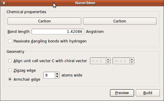
Press the Build button to build the structure.
In order to make sure that the phonon module can detect that the structure is one dimensional, you need to have ~ 7 Å vacuum on both sides of the structure. To this end open .
Increase A-x to 20 Å.
Increase B-y to 30 Å.
and close the widget.
Next, open , and press Apply to center the nanoribbon in the unit cell.
Send the structure to the Script Generator, by using the Send To icon  in the lower right-hand corner of the Builder window.
Defining the phonon calculation
In the following you will optimize the geometry and calculate the Phonon bandstructure and DOS of the nanoribbon using a Tersoff potential.
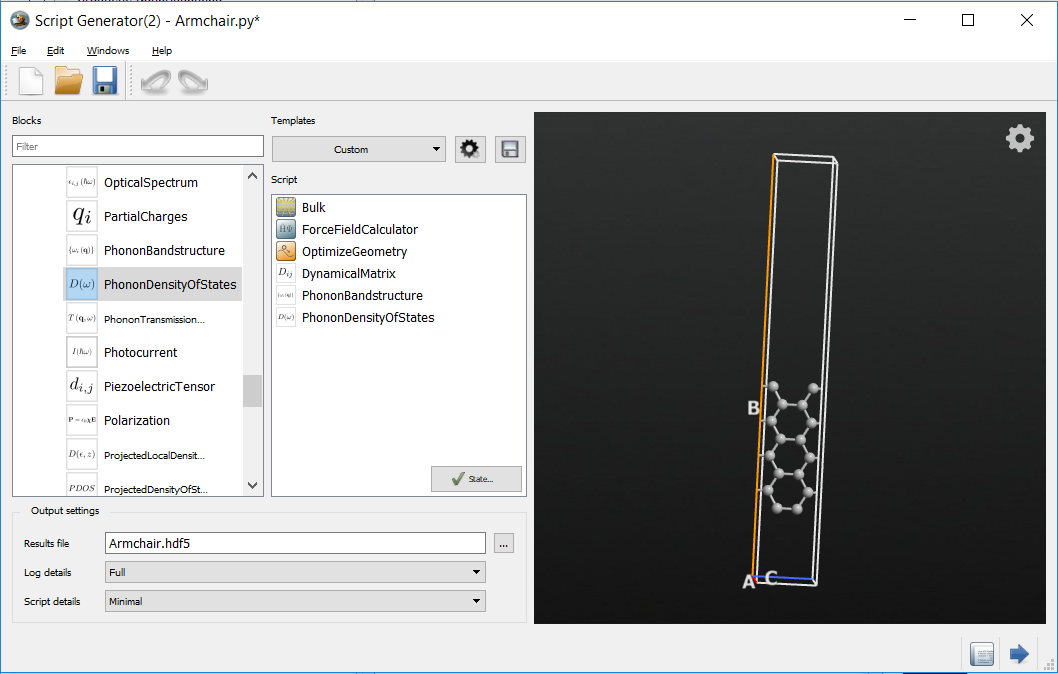
In the Script Generator
Add a ForceFieldCalculator
Add an Optimization > OptimizeGeometry
Add an Analysis > PhononBandstructure
Add an Analysis > PhononDensityOfStates
Change the output file to
armchair.hdf5.
If you take a look at the blocks in the Script Generator, you will notice that a DyamicalMatrix block has automatically been added as the selected phonon analysis functions require the calculation of the dynamical matrix.
Adjusting script components
To set up the calculation parameters, make the following changes:
Double-click the ForceFieldCalculator block and select the Tersoff_C_2010 potential.
Note that depending on the elements present in your configuration you will be able to choose among several potentials. A literature reference is also shown, giving you the possibility to check exactly how the potentials have been generated. It is very important that the potential you will use has been generated for a similar system or for similar conditions as your system.
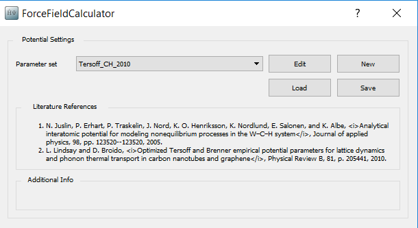
In this case you can immediately see that the Tersoff_C_2010 potential is potentially well suited for your phonon analysis: “Optimized Tersoff and Brenner empirical potential parameters for lattice dynamics and phonon thermal transport in carbon nanotubes and graphene”.
Note
For QuantumATK-versions older than 2017, the ATK-ForceField calculator can be found under the name ATK-Classical.
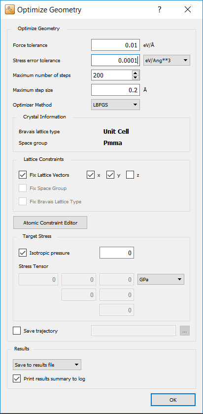
Double-click the OptimizeGeometry and set maximum force to 0.01 eV/Å.
Double-click the PhononBandstructure and set
Points per segmentto 100.Double-click the PhononDensityOfStates. In the q-point Sampling box select
Sampling, uncheck theSyncbox, and setqcto 51.
Transfer the script to the Job Manager (again using the “Send To” icon ) and run the calculation.
Analyzing the Results
The generated output file armchair.hdf5, visible on the LabFloor,
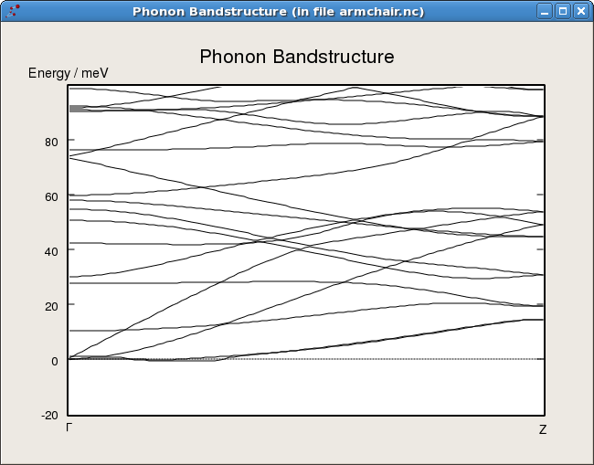
now contains a PhononBandstructure object. Select this PhononBandstructure
object on the LabFloor and press 2D Plot in the plugin panel. Zoom
into the low frequency area to get the figure below.
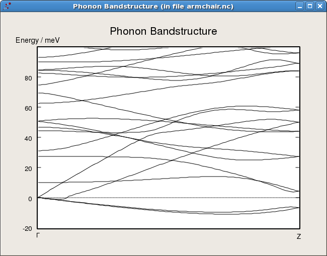
Note the negative bands arising from stress in the nanoribbon which makes it unstable perpendicular to the plane.
Origin of negative phonon bands
The negative bands seen in the phonon spectrum indicate that the structure is at a saddle point and can gain energy by further relaxing. The problem is that you only performed a force optimization and not a stress optimization, thus there is a large stress in the structure and it would like to release the stress by relaxing perpendicular to the graphene plane.
Relaxing the stress in the configuration
In order to relax the stress in the configuration, open the Script Generator again.
Tip
All open tools are available from the Windows menu at the top of each QuantumATK tool.
Next open the OptimizeGeometry block.
Set
Maximum stressto 0.0001 eV/Å 3.Remove check from
zinConstrain cellto allow optimization of the z-component of the cell.
Press OK to close the widget, transfer the script to the Job Manager
and run the calculation. When you open the phonon bandstructure you will see
that the the negative bands are now gone.
The density of states
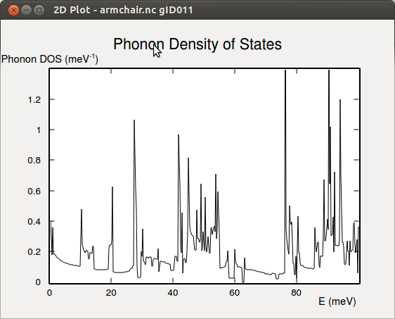
The armchair.hdf5 file also contains the phonon density of state (DOS)
of the armchair nanoribbon with and without stress relaxation. Below the
phonon DOS of the fully (i.e. forces- and stress-) optimized system is shown.
From the phonon DOS it is possible to calculate the free energy, entropy, and
zero point energy of the system. In QuantumATK this is implemented in the
methods freeEnergy(), entropy(), and zeroPointEnergy() of the
PhononDensityOfStates object. The script below shows how to evaluate the
entropy:
 1# Read the last configuration in the output file
 2configuration = nlread('armchair.hdf5', BulkConfiguration)[-1]
 3# Read the last phonon DOS in the output file
 4phonon_dos = nlread('armchair.hdf5', PhononDensityOfStates)[-1]
 5
 6# Define the temperature
 7t = 300*Kelvin
 8
 9# Calculate the entropy
10s = phonon_dos.entropy(t)
11
12# Print results
13print 'Entropy = ', s
Execute the script by dropping it on the Job Manager, and in the Log you will get the output:
Entropy = 4.36888578559 meV/K
Algorithmic Details of the Phonon Calculator
The phonons are calculated from the dynamical matrix of the system. The dynamical matrix is the second derivative of the system, corresponding to the first derivative of the forces. The first derivative of the forces are calculated using a finite difference scheme, where the system is displaced along each degree of freedom in the system, also called frozen phonon calculations.
When you add a new phonon analysis in the Script Generator, it checks if a
dynamical matrix is already present. If this is not the case, a
DynamicalMatrix study object will automatically be added to calculate
the dynamical matrix. The DynamicalMatrix object of a
configuration can be stored in an .hdf5 file and read again to be used
in another calculation.
The details of the calculation of the dynamical matrix is controlled by the parameters in the DynamicalMatrix object.
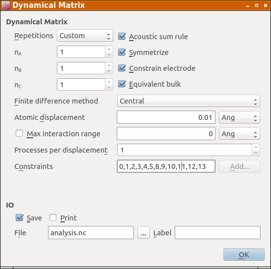
The Repetitions parameter allows you to specify how many repetitions of
the central cell are employed to calculate forces when the atoms in the
central region are displaced. Setting it to Automatic will make sure that
enough repetitions are used, to fit around each atom in the central region a
buffer zone of four times its covalent radius, in which the force derivatives
are taken into account. For the current system the Log file reports:
| Phonon: Automatically detected repetitions = [1 1 5] |
The size of this buffer region can be changed either by using Custom repetitions or by enabling and setting the Max interaction range parameter, which replaces the default buffer radius of four times the covalent radius.
Furthermore, you can change some other parameters, that determine e.g. whether the acoustic sum rule or symmetries are enforced, as well as numerical parameters, e.g. the finitie difference method or the displacement magnitude of the atoms in the central cell.
Note
In most cases the default values should work well. However, if you are using classical potentials with a long interaction range (e.g. potentials which include coulomb interactions), then it might be necessary to increase the Max interaction range to a value somewhat larger than the largest cutoff-radius of the potential. You can normally tell if this is necessary by unchecking Acoustic sum rule and inspecting the acoustic bands at the gamma point. If these bands are not zero, in most cases the maximum interaction range is too low.
K-points used for ATK-DFT and ATK-SE
From QuantumATK-2019.03 onwards, the k-point sampling and density-mesh-cutoff
will be automatically adapted to the given number of repetitions when
setting up the super cell inside DynamicalMatrix. That means you
can specify the calculator settings for the unit cell and use it with any
desired number of repetitions in dynamical matrix calculations.
In previous versions of the code the number of k-points had to be adapted for the dynamical matrix calculation. This is now handled automatically, so the k-points used for phonon calculations do not need to be modified.
Calculating Electrical and Heat Transport for a Graphene Nanoribbon
In this section we will calculate the phonon transmission coefficient for the armchair nanoribbon from which the phonon thermal conductance can be obtained. This will be combined with a calculation of the electron transmission coefficient from which the conductance, Peltier coefficient and electron thermal conductance can be obtained. The different parameters are combined for calculating the thermoelectric figure of merit, ZT. The methodology for the calculations are described in Ref. [1].
Setting up the graphene nanoribbon device
The first step is to build a device geometry from the relaxed armchair
nanoribbon. In the QuantumATK main window select the last configuration in
the armchair.hdf5 file and drag and drop the configuration onto the
Builder.
In the builder perform the following operations:
: Repeat 5 times in C-direction.
: Default values are fine, press
OKto create the device.
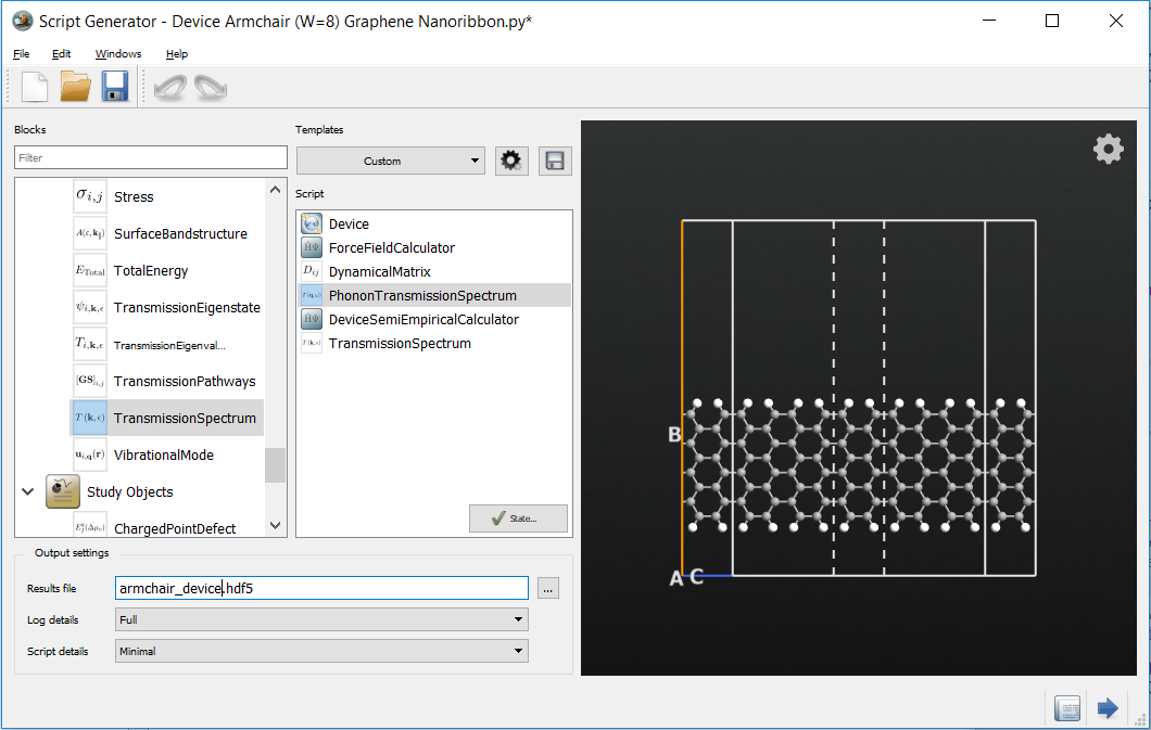
Send the resulting device configuration to the Script Generator.
Defining the transmission calculations
In the following you will setup the phonon and electron transmission calculations. For the phonon calculation you will use the Tersoff potential while using a carbon \(pi\) tight-binding model for the electron transmission calculation.
Add a ForceFieldCalculator.
Add an Analysis > PhononTransmissionSpectrum.
Add a SemiEmpiricalCalculator.
Add an Analysis > TransmissionSpectrum.
Change the output file to
armchair_device.hdf5.
Adjusting script components
To set up calculation parameters, make the following changes:
Double-click the ForceFieldCalculator and select the Tersoff_C_2010 potential. In the results box select
Do not saveand uncheck thePrint results summary to logbox.No changes need to be made to the PhononTransmissionSpectrum.
Double-click the second SemiEmpiricalCalculator and select the
Hamiltoniansettings. In the Basis Set box select the Hancock.C ppPi basis set.
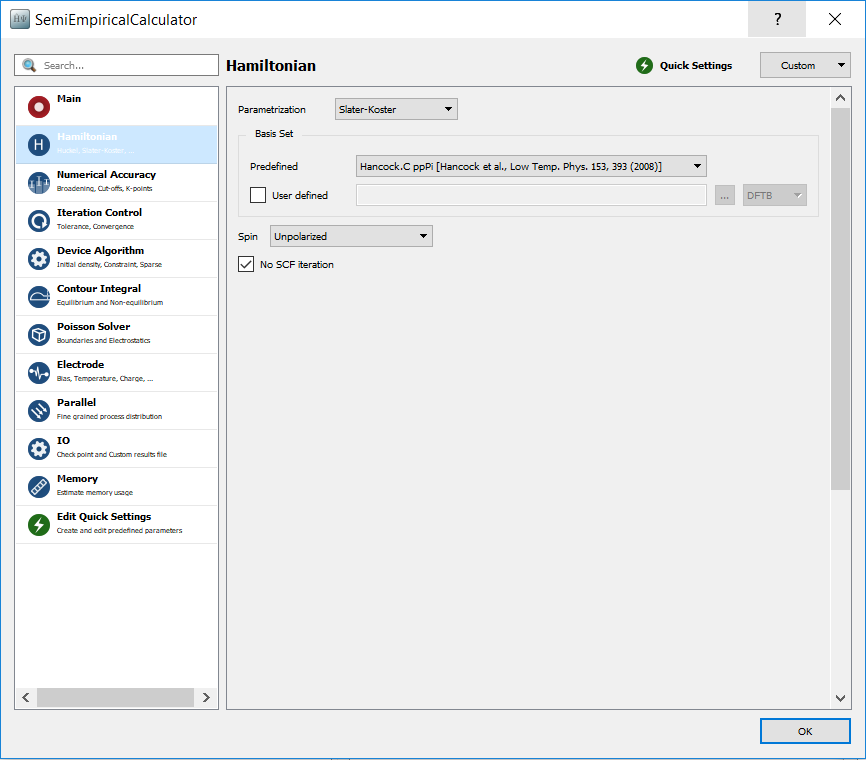
No changes need to be made to the TransmissionSpectrum.
Transfer the script to the Job Manager and run the calculation.
Analyzing the results
Now inspect the result file armchair_device.hdf5 in the QuantumATK
main window. You may select the PhononTransmissionSpectrum and the electron
TransmissionSpectrum and plot them using the Transmission Analyzer or
the 2D Plot analysis plugin.
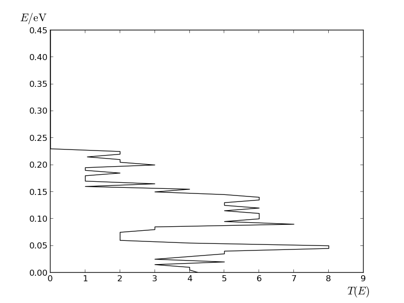
The phonon transmission spectrum of the armchair nanoribbon.
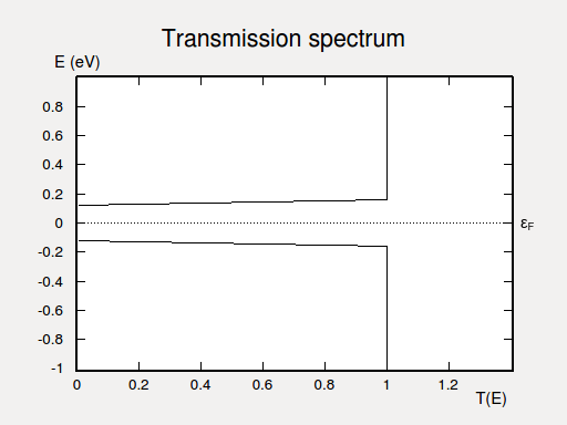
The electron transmission spectrum of the armchair nanoribbon, zoomed into the energy range from -1 to 1 eV.
The thermo-electric figure of merit
In this section you will calculate the linear response transport coefficients of an applied voltage difference (dU) or temperature difference (dT) between the two electrodes. The coefficients are:
The conductance,
The Peltier coefficient,
The Seebeck coefficient,
The heat transport coeficient of electrons, \(\kappa_e\), and phonons \(\kappa_{ph}\),
where \(I_Q = dQ/dT\) is the heat current.
From these coefficients ypu can obtain the thermoelectric figure of merit
which quantifies how efficient a temperature difference can be converted into a voltage difference in a thermoelectric material.
These linear response coefficients are calculated by the Thermoelectric
Coefficients plugin. To perform the calculation, select the
PhononTransmissionSpectrum and the electron TransmissionSpectrum objects
simultanously and press the Calculate button of the plugin.
For an undoped nanoribbon, the Fermi level is in the middle of the band gap. To get a significant Peltier coefficient the Fermi level must be at a band edge, corresponding to a doped nanoribbon. The plugin allows for shifting the Fermi level, and the following shows the result for \(\Delta E_F = 0.08 eV\), corresponding to an n-doped nanoribbon.

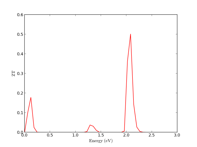
The Thermoelectric Coefficients plugin allows you to plot the different thermoelectric coefficients as a function of the energy. For example, the figure below reports the figure of merit ZT at 300K as a function of the energy. The peaks corresponding to the band edges are clearly visible.
References