In this introductory tutorial, you will learn how to use QuantumATK to
Train custom MACE machine-learned force-fields (ML FFs) using the Workflow Builder for
molecular dynamics (MD), geometry optimization, and other force-field-based simulations for crystal
and amorphous TiSi and TiSi2 structures.
Use the MLFFAnalyzer tool to validate the quality of trained MACE models.
Load trained MACE models into QuantumATK workflows using the Workflow Builder via the
MachineLearnedForceFieldCalculator block.
In recent years, advancements have been made in the world of Machine-Learned Force Fields
(ML-FFs) with the emergence of universal foundation models. One of the current state-of-the-art
potential architectures yielding a good trade-off between performance and accuracy is
MACE[1] - a message-passing Neural Network (MPNN) from which prominent
universal foundation model versions are preinstalled and available for use in QuantumATK.
While such universal models can constitute an excellent calculator in their own right, they
are trained to perform reasonably well within a very broad domain. This means they have been trained on
a large amount of data, and their size limits inference speed. For problems
within a limited application domain, it is possible to train custom MACE models
within QuantumATK. MACE models can be trained either from scratch, which allows you to balance model
size and simulation speed against accuracy, or by fine-tuning foundation models to achieve better
accuracy in a specific application domain while building on top of previous knowledge.
The amount of data needed to train a MACE model depends on the complexity of the
system and the kind of training being conducted. In general, more data is preferred when
training from scratch. However, for fine-tuning from a foundation model, on the order of 100
structures can be enough to reach good accuracy in a specific domain.
In this tutorial, we will demonstrate training MACE models using a small dataset containing a mix
of 241 crystal and amorphous
structures of TiSi and TiSi2. This data was generated and used to train a Moment
Tensor Potential (MTP) in the
Moment Tensor Potential (MTP) Training for Crystal and Amorphous Structures
tutorial. The dataset is available for
download: c-am-TiSi-TrainingSet.hdf5.
For more insight into how the training data was prepared with the ForceFieldTrainingSetGenerator,
see the other tutorial and the ForceFieldTrainingSetGenerator documentation.
Note
This system is chosen for demonstration purposes. For simple systems, the accuracy advantage of MACE over
MTP is not significant. Training an MTP model may be the better choice for this limited use case,
due to its advantages in training speed and simulation performance. MACE is in general expected to
be capable of reaching higher accuracy in complex systems where more traditional ML FFs face limitations.
Note
It is in general advised to do all training of MACE models with 1 GPU using 1 process.
It is similarly recommended to run inference with trained MACE models on GPUs to utilize the
model efficiently. Instructions on how to run a QuantumATK job on GPUs can be found in the
technical notes.
Note
As of Version: Y-2026.03, MACE training and inference with trained MACE models can now utilize
cuEquivariance acceleration on GPU, which can significantly speed up training and inference.
This is always enabled when training on GPU. In order to use cuEquivariance acceleration for
inference with trained MACE models, the appropriate cuEquivariance-enabled model file must be
used. See the MACEFittingParameters documentation for details on generated model file
conventions.
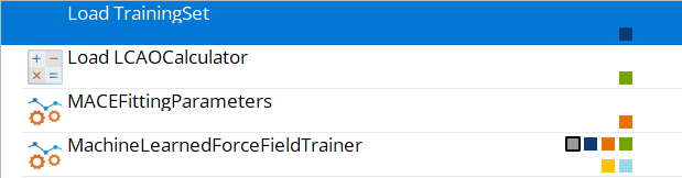
In order to train a single MACE model, we utilize the MACEFittingParameters and
MachineLearnedForceFieldTrainer blocks in the Workflow Builder.
This results in a workflow with the following structure, assuming training set data has previously
been generated and a calculator is provided. The calculator must be consistent with the one used to
generate the training data and is needed to compute isolated atom energies for each element in the
system. Isolated atom energies are the DFT energies of single atoms computed in isolation, which
are used to shift the total energy predictions during training. Subtracting the sum of these
isolated atom energy constants from the total energy of each structure and focusing strictly
on learning the interaction effects improves training stability and model generalization.
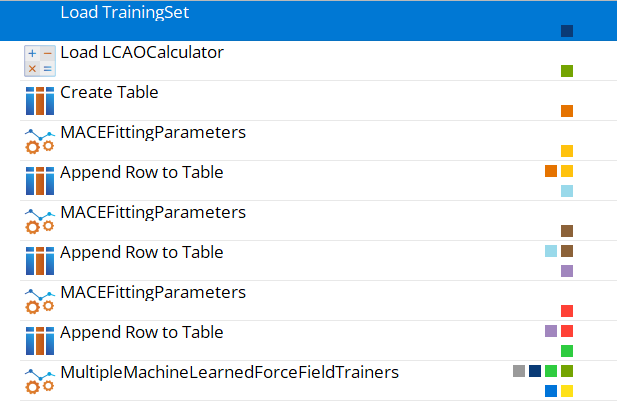
It is also possible to train multiple models - defined via MACEFittingParameters and/or
MomentTensorPotentialFittingParameters blocks appended to a single Table block - in the same
workflow by using the MultipleMachineLearnedForceFieldTrainers blocks. This allows you to compare
different models trained on the same training data with differing fitting parameters easily.
This results in a workflow with the following structure, assuming training set data has previously been
generated:
Both approaches will be demonstrated in this tutorial.
Note
For large-scale MACE training with large training sets, it is in general recommended to only train a single
model per QuantumATK job submission due to the time required to train a model. To efficiently
train, validate, and compare multiple models, it is recommended to train each model in a separate job
and manually collect the resulting MachineLearnedModelEvaluator objects in a single
MachineLearnedModelCollection object for convenient comparison in the MLFFAnalyzer.
Load TrainingSet, containing the precomputed training data. This block is loaded from file in this
tutorial but can also be explicitly created previously in a workflow, if not yet assembled.
Set the correct path to the downloaded TrainingSet object via the
Load from file button and navigate to the correct file and object. The training set contains
a mix of crystal and amorphous structures of TiSi and TiSi2 with DFT energies,
forces, and stresses.
Load LCAOCalculator, for calculating isolated atom energies during training. Here we load
it from the same data file, but it can also be set up from scratch - it is important that
this calculator is consistent with how the training data was generated (e.g., same pseudopotentials,
basis sets, and DFT settings).
Set the correct path to the downloaded calculator via the Load from file button and navigate
to the correct file and object.
MACEFittingParameters, defining the model, dataset, and training parameters
to apply during the model training.
MachineLearnedForceFieldTrainer, coordinating the training.
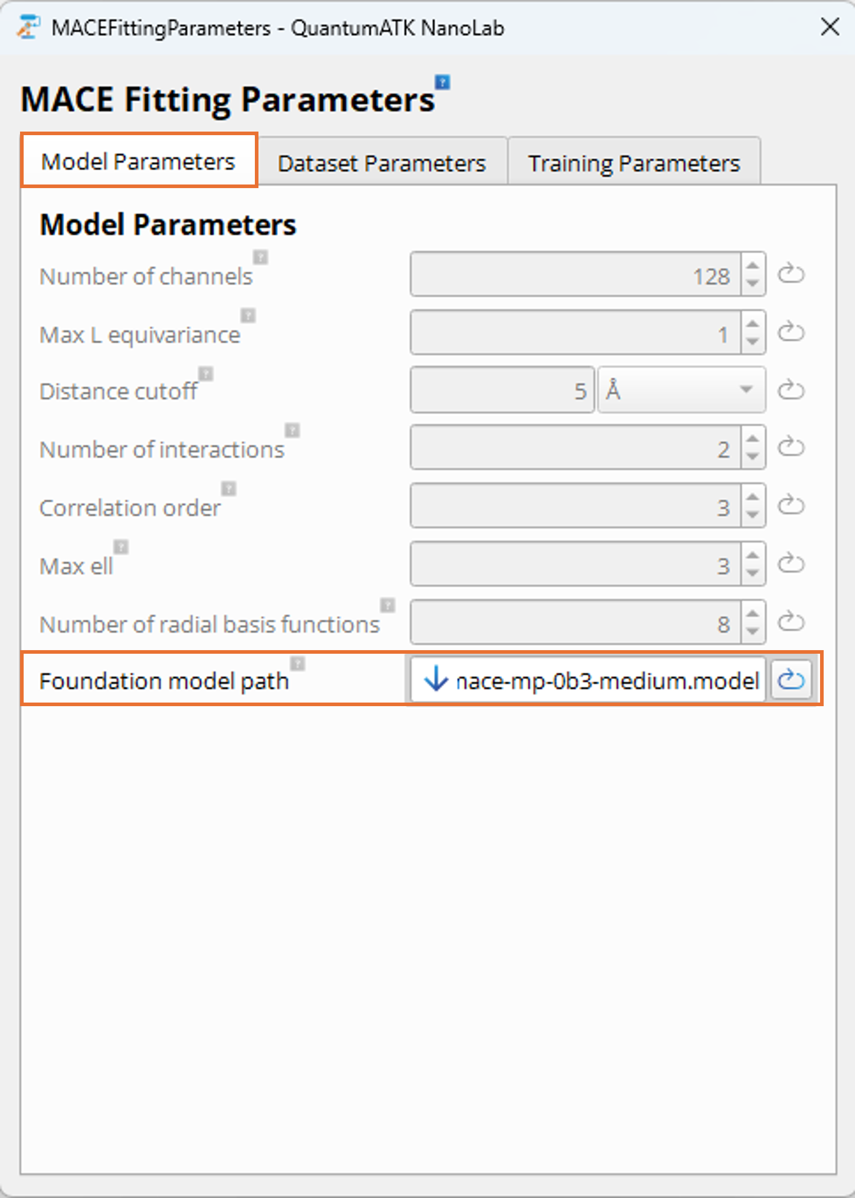
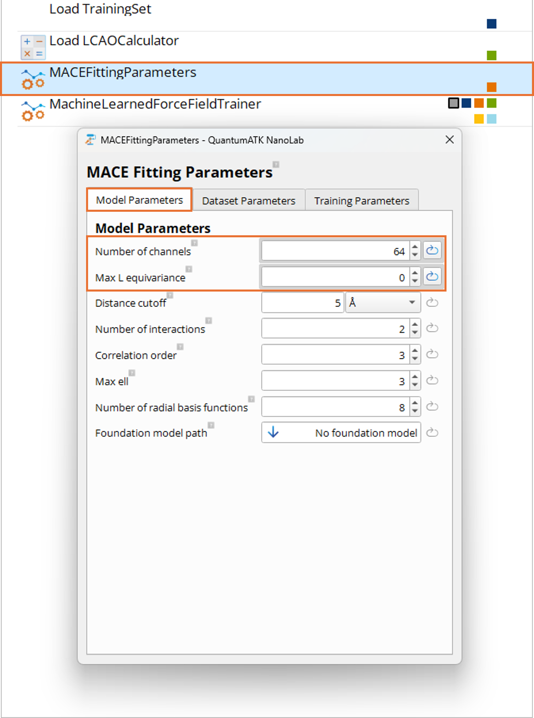
Double-click on the MACEFittingParameters block to configure the training. The block has three tabs:
Model Parameters, Dataset Parameters, and Training Parameters.
Model Parameters Tab:
When training from scratch, the model parameters define the architecture of the MACE model and have a significant
impact on the potential accuracy, speed, and size of the resulting model.
The most important parameters for model size, speed, and accuracy are Max L equivariance,
Number of channels, and Distance cutoff. For this tutorial, we set these parameters to values
yielding a smaller, faster model than those used for foundation models.
Set Max L equivariance to 0 for this example (corresponding to “small” or “L0” foundation MACE models).
Setting it to 1 gives “medium”/”L1” models and 2 gives “large”/”L2” models. This parameter has
the largest impact on computational speed and accuracy of a trained model.
Set Number of channels to 64 for this example, which is a lower setting than used by foundation
models. 64 or even lower values are suitable for this demonstration and in general for smaller,
specialized, performant models. Higher values (e.g., 128) improve accuracy but increase training
time, model size, memory usage, and inference time.
The Distance cutoff is kept at the default 5.0Angstrom. This controls the cutoff radius for the local
environment.
The remaining parameters under the Model Parameters tab in general have smaller impact on accuracy and
performance and can typically remain at their default values. Expert users can experiment with these
settings to further optimize the model. For more details on all parameters, see the
MACEFittingParameters documentation.
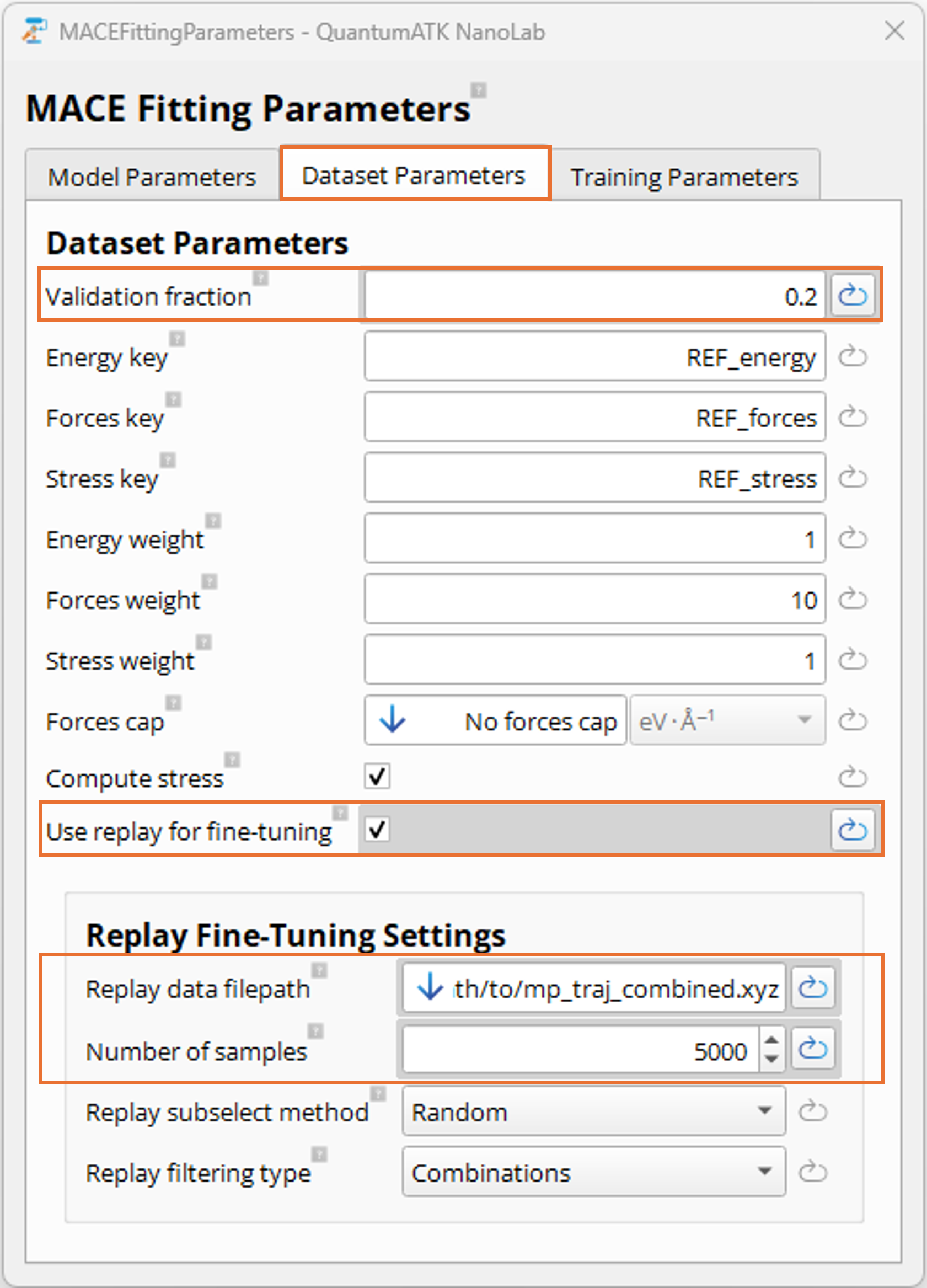
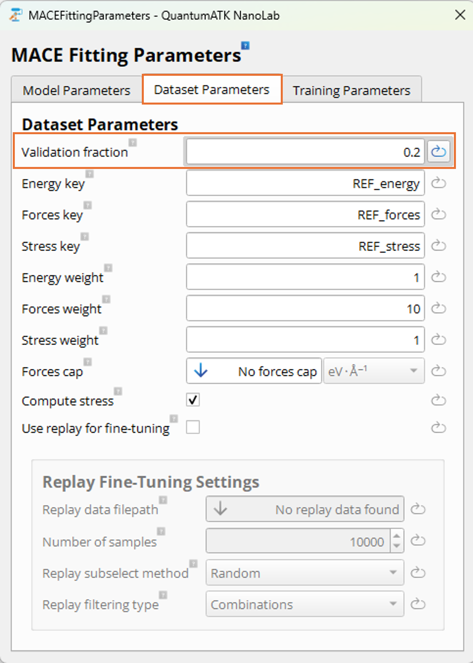
Dataset Parameters Tab:
In the Dataset Parameters tab, you can configure how the loss function weights and dataset parameters
should be set for the
training. The default settings are typically a good starting point, but since the training set is small
we make a change to ensure the training process is stable and converges to a decent model
for this tutorial.
Set Validation fraction to 0.2 to use 20% of the training data as a validation set during
training. This is important to maximize the chance of a successful training process and
avoid overfitting or undersampling in certain regions of the configuration space when using a small dataset.
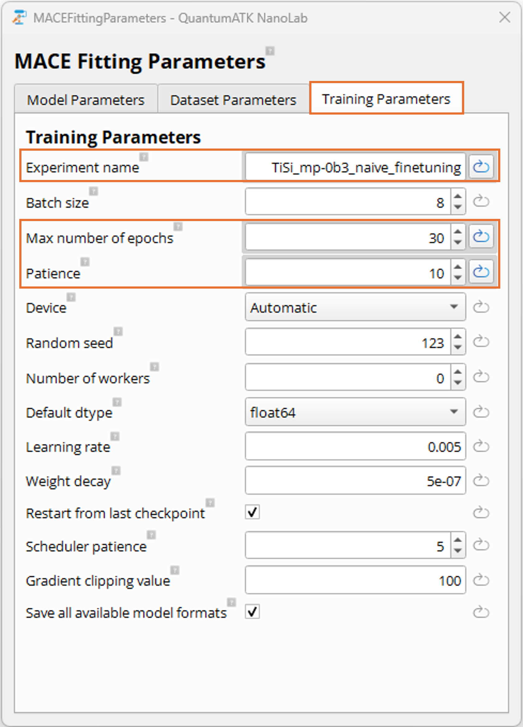
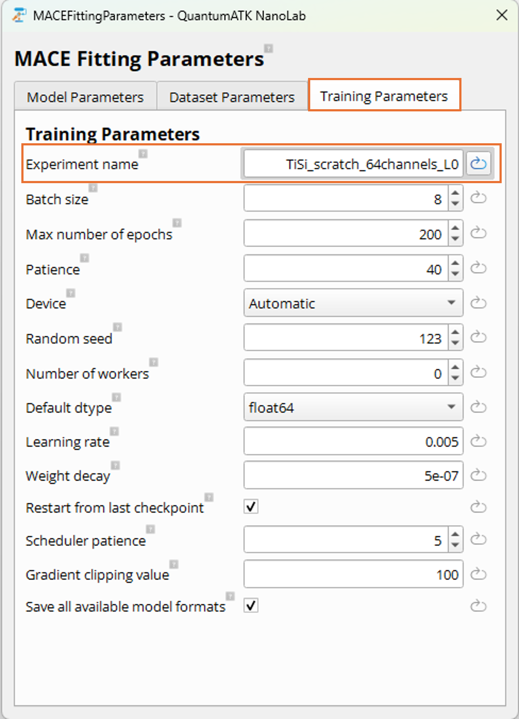
Training Parameters Tab:
In the Training Parameters tab, you can configure the training process. The most important parameter
in this tab
is the Experiment name which should be set as a meaningful, unique name describing the training run and will
constitute the base of the resulting model file name. Other influential parameters include the
Max number of epochs and Patience parameters, which control how long the training runs and early stopping criteria.
These and additional parameters can be explored in the MACEFittingParameters documentation.
For this tutorial, we rely on defaults apart from these settings:
Set Experiment name to TiSi_scratch_64channels_L0 to indicate the system, type of training (scratch),
and the key model parameters used.
The MachineLearnedForceFieldTrainer block coordinates the training process.
The Train test split and Random seed parameters of the block can be set to control the ratio and
seed of the train/test split. In this tutorial, we rely on the default settings only.
Click on the Send content to other tools button and choose Job as a script
to send the workflow to the Jobs tool.
In the Job Manager, configure the job to use 1 MPI process and 1 GPU. Instructions on how to run on GPUs
can be found in the technical notes. If running with GPU enabled is not an option,
it is possible to train on CPU, but this is not recommended due to the significantly longer training time.
Submit the job. Using a single node with a single GPU (NVIDIA A100), the training took approximately 10
minutes when writing this tutorial.
Tip
Monitor the training progress in the streamed output log. Loss scores (in the form of Huber loss scores) are
reported after each epoch.
Fine-tuning a foundation model can improve accuracy for a specific domain while
benefiting from the general relationships learned by the original model. The foundation model architecture
is fixed, so the model size is tied to the foundation model used. However, fine-tuning requires
less training data than training from scratch in order to achieve a model with good accuracy.
Fine-tunable foundation models are not included in the QuantumATK installation.
Any universal MACE model to be fine-tuned must first be downloaded and then provided to the
workflow. Due to file size, it is beneficial to store the model on a cluster
and reference it there rather than copying it with each job submission.
The workflow structure is similar to training from scratch, but with modified MACEFittingParameters.
Update the filepaths in the Load TrainingSet and Load LCAOCalculator blocks to point to the correct
locations of the downloaded training set and calculator objects, as described in the previous section.
Double-click on the MACEFittingParameters block. In the Model Parameters tab:
Set Foundation model path to the location where you placed the downloaded
mace-mp-0b3-medium.model (or a similar foundation) model file. If running the job on a cluster,
the path set here should be the path to the file on the cluster. Otherwise, update the path to the
local file location. The path provided here in the workflow is just
a placeholder and needs modification before the job can run.
The other model parameters that control the architecture of the model are inherited from
the foundation model and cannot be changed when fine-tuning. They therefore are ignored
when the Foundation model path is set. This means that the resulting fine-tuned
model will have the same architecture, size, and speed as the foundation model used.
Navigate to the Dataset Parameters tab and make the same change as for the
training-from-scratch workflow:
Set Validation fraction to 0.2 to use 20% of the training data as a validation set during
training. This is important to maximize the chance of a successful training process and
avoid overfitting or undersampling in certain regions of the configuration space when using a small dataset.
Navigate to the Training Parameters tab:
Set Experiment name to a unique name like TiSi_mp-0b3_naive_finetuning to identify
this training run.
Since the model is being fine-tuned from a foundation model, it is recommended to reduce
the number of epochs to avoid over-fitting to the new domain and thereby degrading general
learned relationships from the foundation model. Therefore, in this tutorial, we set
Max number of epochs to 30 and the Patience to 10. The optimal number of
epochs for fine-tuning depends on the size and quality of the new training data and it
is recommended to experiment with this parameter for your specific application. In general,
a good indicator of when a model is sufficiently fine-tuned is when the validation loss
plateaus, which can be inspected in the MLFFAnalyzer after training. If the validation
loss (i.e. the combined Huber loss optimization score) has converged or no longer
improves significantly it is a good indication that the number of epochs was sufficient
and the training has converged.
Submit the job following the same procedure as before. Using a single GPU (Nvidia A100),
the training took approximately 4 minutes when writing this tutorial.
Note
During naive fine-tuning, the foundation model is trained further on new data. While this can
significantly improve accuracy within the new domain, it carries the risk that some general
knowledge encoded in the original foundation model may be forgotten, especially if the new
dataset is very different from the original training data.
Multihead Replay Fine-tuning of Foundation MACE Models
Multihead Replay Fine-tuning is a more refined approach to fine-tuning.
Unlike naive fine-tuning, this method uses both the foundation model and the original training
data used to train the foundation model in order to preserve the original knowledge. At the
same time, it also adapts to the new domain by training on the new data.
The model trains on multiple model “heads” with separate readout layers but sharing most model weights. One head
retrains on a subset of the original training data, while another
head trains on your new data. This minimizes the risk of “forgetting” the original knowledge
while adapting to the new domain.
The workflow structure is similar to training from scratch, but with modified MACEFittingParameters.
Update the filepaths in the Load TrainingSet and Load LCAOCalculator blocks to point to the correct
locations of the downloaded training set and calculator objects, as described in the previous section.
For multihead fine-tuning with MP MACE models, you need to download the original training data,
at the time of the Version: Y-2026.03 release available at:
mp_traj_combined.xyz[2][3]
Double-click on the MACEFittingParameters block. In the Model Parameters tab:
Set Foundation model path to the location where you placed the downloaded
mace-mp-0b3-medium.model (or a similar foundation) model file. If running the job on a cluster,
the path set here should be the path to the file on the cluster. Otherwise, update the path to the
local file location. The path provided here in the workflow is just
a placeholder and needs modification before the job can run.
The other model parameters that control the architecture of the model are inherited from
the foundation model and cannot be changed when fine-tuning. They therefore are ignored
when the Foundation model path is set. This means that the resulting fine-tuned
model will have the same architecture, size, and speed as the foundation model used.
Navigate to the Dataset Parameters tab and use the same settings as in the previous section
for Validation fraction:
Set Validation fraction to 0.2 to use 20% of the training data as a validation set during
training. This is important to maximize the chance of a successful training process and
avoid overfitting or undersampling in certain regions of the configuration space when using a small dataset.
Then, make the following adaptions for enabling and configuring multihead replay fine-tuning:
Select and click the checkbox for Use replay for fine-tuning to enable multihead replay
fine-tuning. This will enable additional parameters to set in the Replay Fine-Tuning Settings.
In the Replay Fine-Tuning Settings make the following adaptions:
Set Replay data filepath to the location where you
downloaded the mp_traj_combined.xyz original MP foundation model data file. Update this
path to your local or cluster (recommended) location for the file. The one provided here
in the workflow is just a placeholder and needs modification to run.
Set Number of samples to 5000 to reduce the training time for this tutorial.
For achieving the best results, it is in general recommended to use 10000+ samples. The more elements and
element combinations included in the user training data, the more beneficial it is to
utilize a larger number of samples from the original training data to preserve the
foundation model’s knowledge within the same domain and keep the number of required new data configurations low.
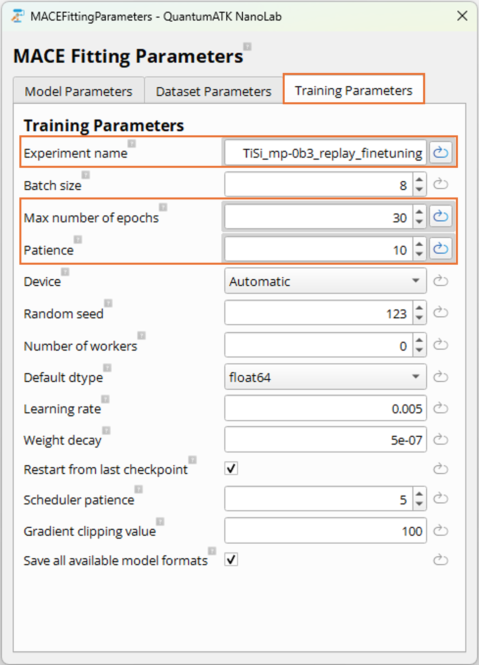
Navigate to the Training Parameters tab.
Set Experiment name to a unique name, such as TiSi_mp-0b3_replay_finetuning,
to identify this training run and resulting models.
Since the model is being fine-tuned from a foundation model, it is recommended to reduce
the number of epochs to avoid over-fitting to the new domain and thereby degrading general
learned relationships from the foundation model. The effect of this will be smaller than
for naive fine-tuning. In this tutorial, we again set
Max number of epochs to 30 and the Patience to 10. The optimal number of
epochs for fine-tuning depends on the size and quality of the new training data and it
is recommended to experiment with this parameter for your specific application. In general,
a good indicator of when a model is sufficiently fine-tuned is when the validation loss
plateaus, which can be inspected in the MLFFAnalyzer after training. If the validation
loss (i.e. the combined Huber loss optimization score) has converged or no longer
improves significantly it is a good indication that the number of epochs was sufficient
and the training has converged.
Submit the job. Using a single GPU (NVIDIA A100), the training took approximately
30 minutes when writing this tutorial.
Tip
Due to the large file sizes, it is strongly recommended to store the foundation model
and original training data files on the cluster where training will occur, to avoid
handling large file transfers as part of the Job submission.
Validation of Trained Models Using the MLFFAnalyzer
After training, it is essential to validate model accuracy on unseen data. This happens
automatically when using the MachineLearnedForceFieldTrainer and
MultipleMachineLearnedForceFieldTrainers blocks, where a 1-train_test_split
ratio of the passed TrainingSet data is used as a test set with the trained model
and errors are computed with reference to the labelled DFT for the corresponding configurations.
The results are saved to the results hdf5-file as a MachineLearnedModelEvaluator
object, when training with the MachineLearnedForceFieldTrainer block, or as a
MachineLearnedModelCollection object, when training with the
MultipleMachineLearnedForceFieldTrainers block. These contain the computed errors in terms of
RMSE, MAE, and R2-score for each quantity (energy, forces, and stress), as well as
the predicted vs reference values for scatter plots.
Navigating to the Lab Floor, the test results of the trained models can be
inspected.
Since training MACE models can take a significant amount of time, it is in general recommended
to train models individually and collect the resulting MachineLearnedModelEvaluator
objects in a single MachineLearnedModelCollection object for convenient
comparison in the MLFFAnalyzer.
For this tutorial, an additional workflow containing all previous model trainings
utilizing a MultipleMachineLearnedForceFieldTrainers block has been
created for convenient comparison. The workflow is available for
download: Train_multiple_models.hdf5.
Running this workflow results in a MachineLearnedModelCollection object
containing the results for all three models trained in this tutorial, which can be
opened in the MLFFAnalyzer for comparison. This is included here to showcase some
of the capabilities of the MLFFAnalyzer for inspecting and comparing MACE training results.
Running this combined workflow using a single GPU (NVIDIA A100), the training took approximately
45 minutes when writing this tutorial.
Note
Note that the models trained in this tutorial have not been trained with the optimal
settings for achieving the highest accuracy, but rather with settings that allow for a quick demonstration
of the training and validation process. For achieving the best results, it is recommended to experiment
with the MACEFittingParameters hyper-parameters, with more initial data, and ensure convergence. Similarly, it is
important to remember that while models can
always be optimized via hyper-parameter tuning, the accuracy of a model is ultimately limited by the quality,
diversity, and size of the training data used. For achieving the best all-round models for production, it is
therefore important to consider all aspects.
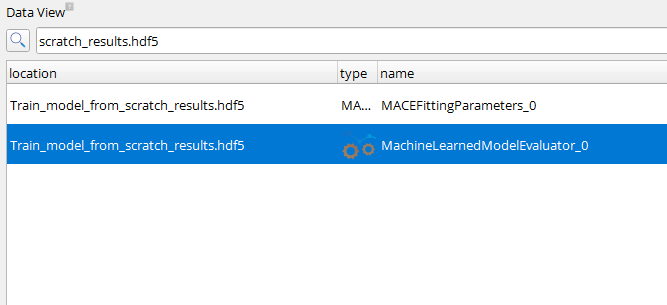
Starting with a single model trained from scratch with the
MachineLearnedForceFieldTrainer, the results are stored in the location
Train_model_from_scratch_results.hdf5 in the MachineLearnedModelEvaluator object.
If not running the training yourself, you can also download the results file
here: Train_model_from_scratch_results.hdf5,
or alternatively transfer them from the zip file to your project.
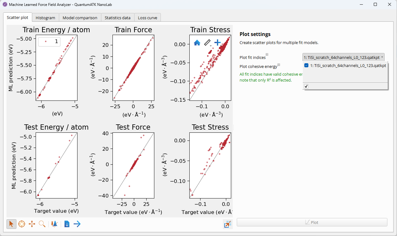
Double-clicking the object opens the results in the MLFFAnalyzer tool.
On the Scatter Plot tab, you can inspect the predicted vs reference values for
energy, forces, and stress for the trained model. In the dropdown menu on the right-hand-side,
the relation between the fit index (here the number 1) and the model filename (in its
non-cuEquivariance base form) is shown. For a single model trained with the
MachineLearnedForceFieldTrainer, there is only one fit index and model file.
For multiple models trained with the MultipleMachineLearnedForceFieldTrainers,
there are multiple fit indices corresponding to each model file, which can be
selected in the dropdown menu to inspect the results for selected models
simultaneously.
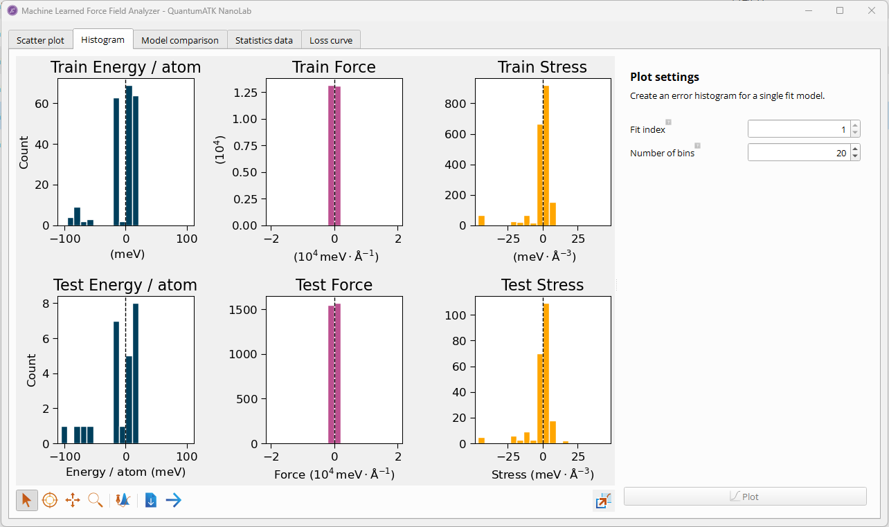
On the Histogram tab, you can inspect the distribution of errors for energy,
forces, and stress. This helps identify any systematic biases or outliers in the
predictions. This tab only works for individual models. If opening model results
in a MachineLearnedModelCollection object containing multiple models,
individual distributions can be accessed via the fit index menu.
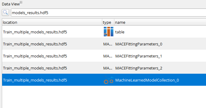
Focusing now on the results from the workflow with multiple models trained with
the MultipleMachineLearnedForceFieldTrainers, the results are stored in the location
Train_multiple_models_results.hdf5 in the MachineLearnedModelCollection object.
If not running the training yourself, you can also download the results file
here: Train_multiple_models_results.hdf5,
or transfer them from the zip file to your project.
Double-clicking the object opens the results in the MLFFAnalyzer tool.
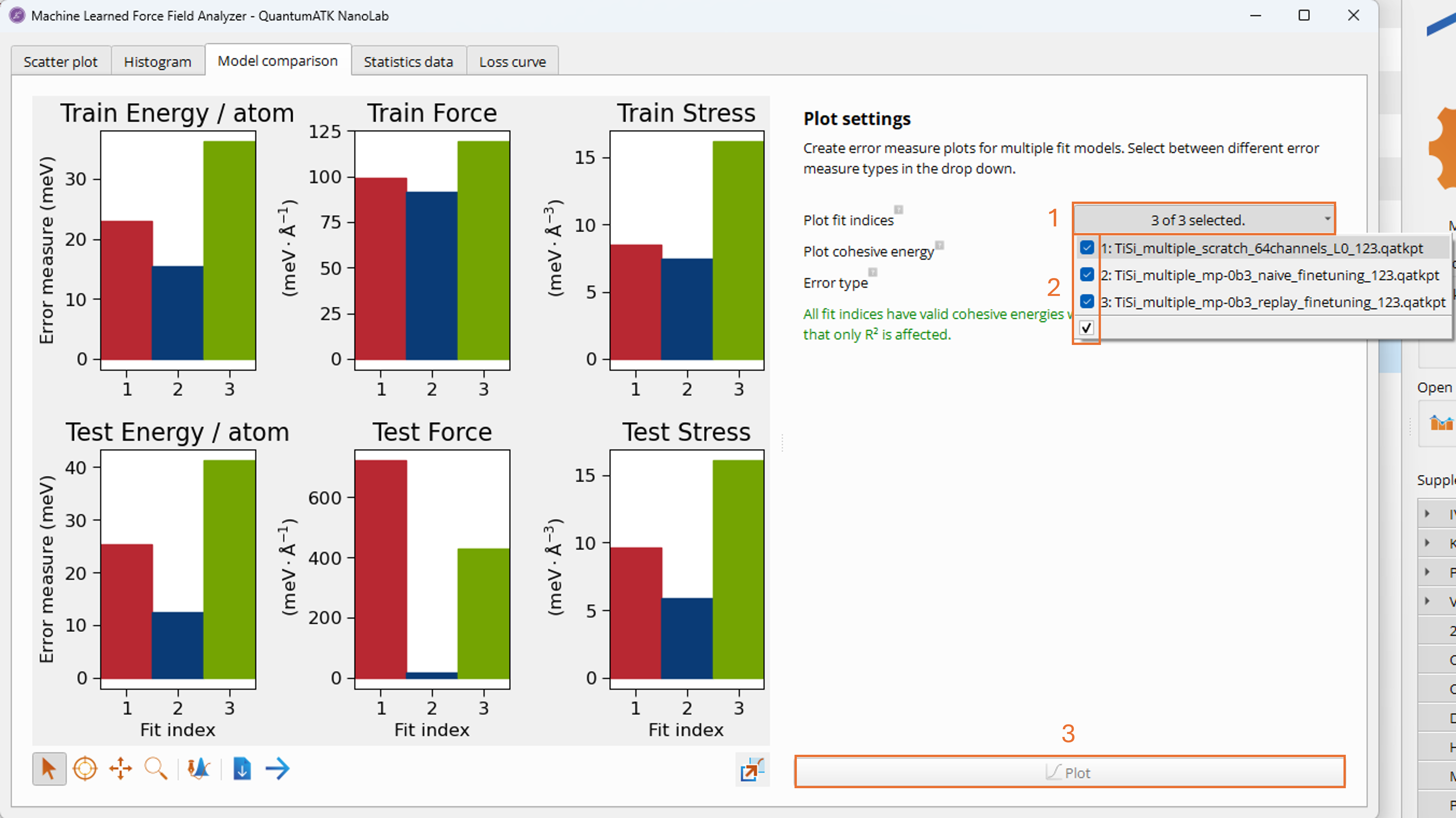
On the Model comparison tab, energy, forces, and stress errors are reported across
the training set and the test set in terms of the chosen error metric (RMSE by default)
in appropriate units.
By clicking on the Plot fit indices dropdown menu (1), it is possible to select which
model fit indices to plot simultaneously. Choosing all three (2) and clicking the Plot
button (3) updates the plots to grant easy visual comparison of the errors across the
different models.
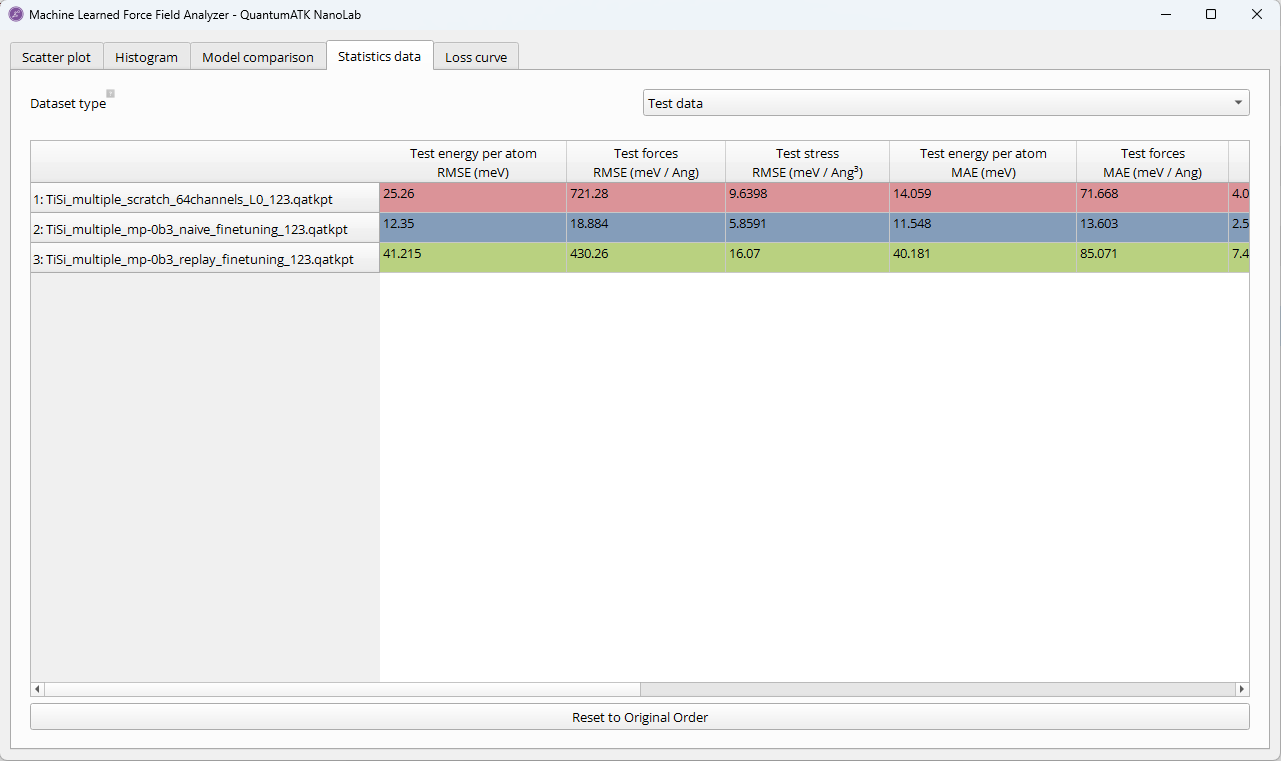
On the Statistics data tab, a table of all summarized error measures across
quantities, data sets, and trained models and their corresponding fit indices is
shown for complete access to the detailed accuracy metrics on the sample data sets.
By default, models are sorted by fit index.
By clicking on
any column header, the rows are sorted in descending order according to the error scores in that column.
Clicking the same header again reverses the sorting to ascending order.
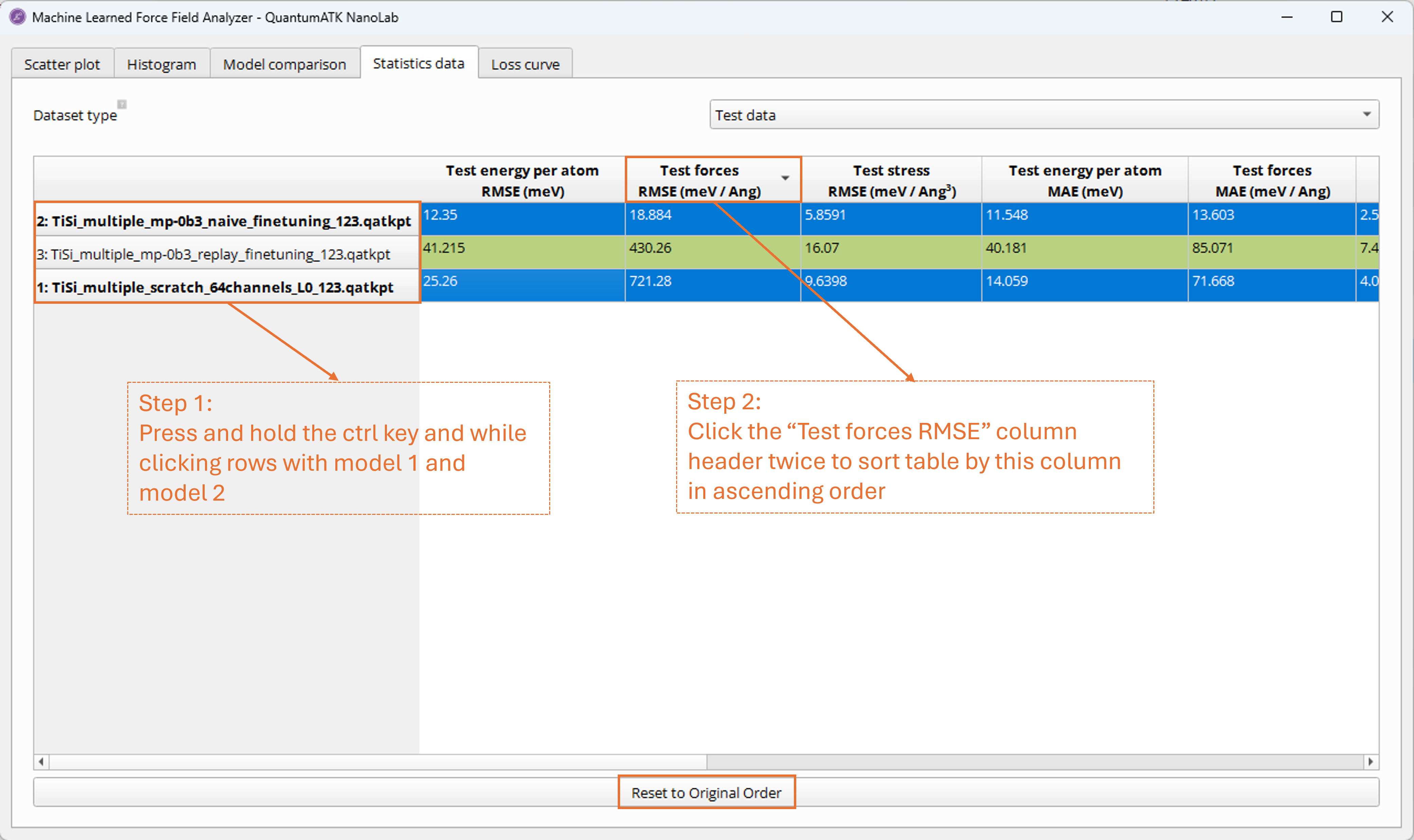
In the table, it is also possible to click anywhere in a table row for a specific
model (or multiple models if holding down the ctrl key while clicking repeatedly)
and then use the column sorting in order to easily track the comparative
performance of specific models across different error metrics and data sets. The highlighted
model rows are shown in bold text.
The table can be reset to the original order by clicking the Reset to Original Order
button.
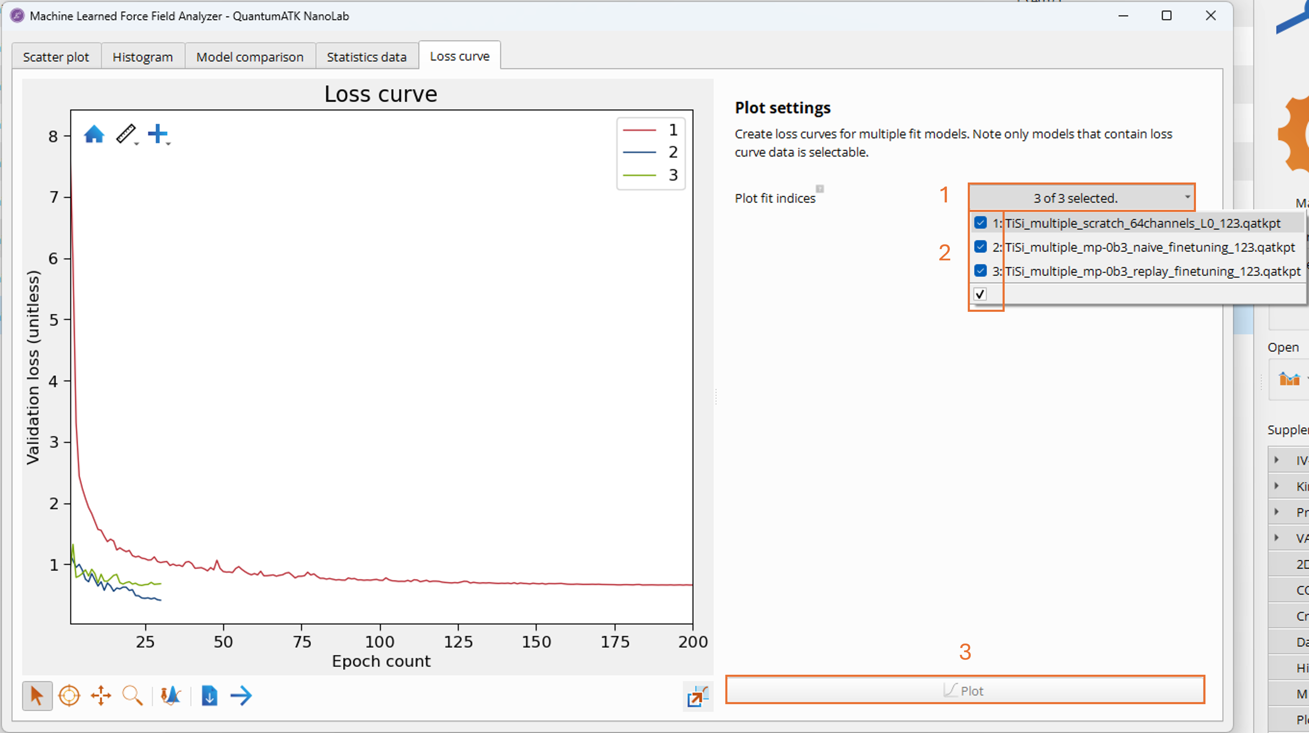
On the Loss curve tab, the validation loss (a unitless loss score combined over the
energy, forces, and stress quantities with the associated weights from the
MACEFittingParameters → Dataset Parameters) is plotted against the training
epochs for each model. By clicking on the Plot fit indices dropdown menu (1), it is
possible to select and add additional models (2) to plot via the Plot button (3),
allowing you to visually compare the training process and convergence behavior of
the different models.
Low RMSE values: Lower is better, but acceptable values depend on your application.
Similar train and validation errors: Large differences may suggest overfitting or
undersampling of certain regions of the configuration space in the data splits.
Points near the diagonal: In scatter plots, this indicates good predictions.
Note
Validation errors are typically slightly higher than training errors because the model
has not seen the validation data during training. This is expected and indicates the model
is not severely overfitting or undersampled in any of the spanned regions of the configuration space.
If you have trained multiple models, you can compare them by:
Opening each model’s MachineLearnedModelEvaluator or the combined models’
MachineLearnedModelCollection results in the MLFFAnalyzer.
Comparing RMSE values across models.
Noting trade-offs between accuracy and model size/speed (tied to model architecture).
In general, it can be expected that:
Fine-tuned models achieve better accuracy than models trained from scratch.
Multihead fine-tuning helps retain general knowledge while adapting to the new domain.
Models from scratch may be faster but require more training data for comparable accuracy.
Comparing models only on a small test set gives an initial indication of model performance compared
to other models, but it is recommended to further validate models by running them in
production-like test simulations using Molecular Dynamics to ensure model stability and expected
behavior over long simulation times. For any model considered to be used for production simulations,
this is a critical step in the validation process to ensure reliable simulations. Setting up such a
simulation for either testing a newly trained model or using a trusted MACE model in production is
described in the following section.
Using Custom MACE Models with Calculators in the Workflow Builder
Once a model has been trained, 1 or 3 .qatkpt MACE model files are created, which can be used as
TorchXPotentials in QuantumATK workflows. If training with GPU, 3 versions of the model file
are created by default: a standard version usable on both CPU and GPU, and 2 cuEquivariance-optimized versions
(with _cue_fp32 or _cue_fp64 suffixes in the filename) optimized specifically for very fast performance
but locked to either 32-bit or 64-bit float precision and GPU usage. If a training was conducted without GPU,
only the standard version of the model file is created, which can still be used on GPU but without cuEquivariance
acceleration.
A sample workflow showing how to set up a calculator with a custom MACE model is
available for download, here in the form of a simple MD
simulation: Molecular_dynamics_scratch_model_usage_example.hdf5.
To run it, the trained model from scratch is also available for download. The universal form of the model usable on
both GPU and CPU but without cuEquivariance acceleration is available here: TiSi_scratch_64channels_L0_123.qatkpt.
The 32-bit cuEquivariance-optimized version of the model is available here: TiSi_scratch_64channels_L0_123_cue_fp32.qatkpt.
In a real model validation workflow, you should test on one or more relevant benchmark systems and
over long timescales, to ensure that the model is stable and behaves as expected in production simulations.
The procedure of using trained MACE models in calculators in the Workflow Builder is the same
whether you are setting up a quick test or a long production simulation:
Navigate to the Workflow Builder and open the example workflow.
It contains a simple TiSi configuration and a simple NVT MD block.
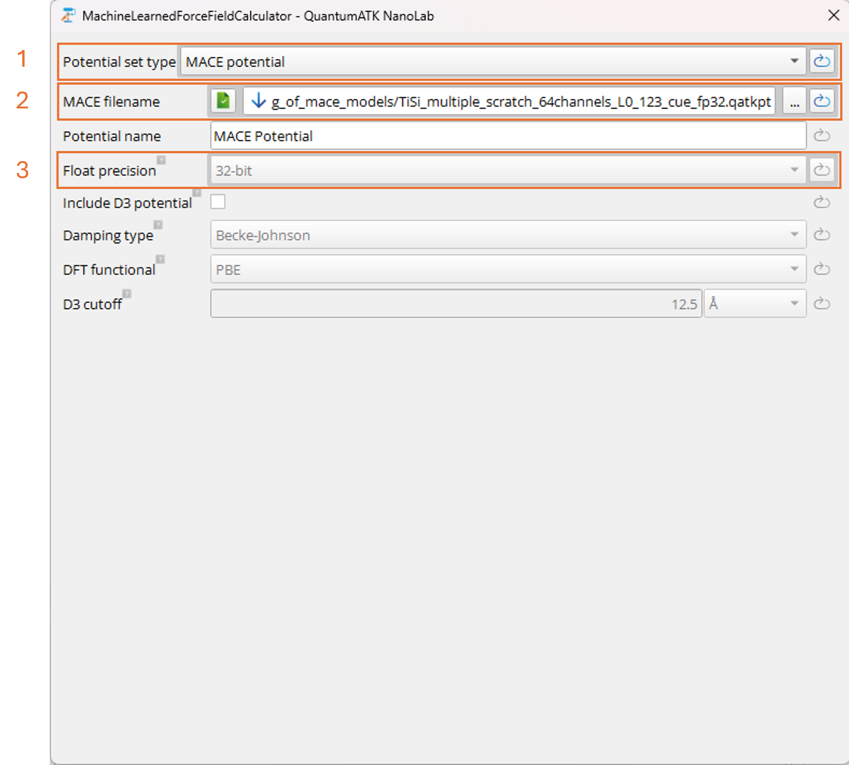
Double-click on the Set MachineLearnedForceFieldCalculator block:
Set Potential set type to MACEpotential (1).
In the MACE filename field, click the ... button to browse to the location of your trained or
downloaded MACE model file (2). If running the simulation on CPU, select the standard version of the
model file without the cuEquivariance suffix. If running the simulation on GPU, either version
can be used. Both the standard version on GPU and the cuEquivariance-optimized version on GPU are significantly
faster than the standard version on CPU. The fastest performance is achieved with the
cuEquivariance-optimized version on GPU.
If using the standard model version, the Float precision can be set (3). For Molecular Dynamics
simulations, it is recommended to use 32-bit precision for improved speed. For the
cuEquivariance-optimized version, the float precision is locked and tied to the loaded model file.
Send the workflow to the Job Manager and submit the job. If using the standard model, GPU
will be used if enabled. If using the cuEquivariance-optimized model, it is required that GPU
is enabled.
When setting up your own MACE trainings, the following parameters have the largest impact:
Model Architecture (Training from Scratch Only):
Max L equivariance:
0 (“small”/”L0”): Fastest, suitable for many systems.
1 (“medium”/”L1”): Better accuracy, slower - corresponds to the architecture of
the current foundation models at the time of the Version: Y-2026.03 release.
Start with 0 for training smaller, performant models; increase if
accuracy is insufficient.
Distance cutoff:
Typically 5-6 Å, range of 4-7 Å.
Larger values improve accuracy for long-range interactions but
increase computational cost.
Number of channels:
Typically 64 or 128 for production models.
Lower values (8-32) create faster but less accurate models.
Higher values improve accuracy with diminishing returns.
Dataset Parameters:
Loss function weights:
Balance energy, forces, and stress importance in the loss function during training.
Forces should typically be weighted higher than energy.
Adjust based on which quantities are most important for your application.
Training Parameters:
Max number of epochs:
Number of epochs that a model can at maximum undergo during training.
Rule-of-thumb as a starting point: \((N_{\mathrm{config}} \times N_{\mathrm{epochs}}) / N_{\mathrm{batch}} \approx 200{,}000\)
gradient updates.
Here, \(N_{\mathrm{config}}\), \(N_{\mathrm{epochs}}\), and \(N_{\mathrm{batch}}\)
correspond to number_of_configurations, max_epochs, and batch_size.
The Patience parameter can stop training early if validation loss converges.
Random seed:
Controls random initialization and train-test split. For reproducibility, set to
a fixed value.
For critical applications, train multiple models with different seeds. This is
achieved by running the same workflow multiple times with different Random seed values in the
Training Parameters tab in the MACEFittingParameters block. It may also
be beneficial to train multiple models with different train-test data splits of the
configurations data by sampling different values for the Random seed parameter of the
MachineLearnedForceFieldTrainer block.
The resulting models can then be compared in the MLFFAnalyzer to select the
best performing model for production simulations.
Batch size:
Larger batch sizes generally result in faster training.
Maximum batch size may be limited by GPU memory and model size.
When increasing batch size, it is recommended to also increase the learning rate proportionally
to maintain training stability and convergence speed.
Fine-tuning Parameters:
Foundation model path: Path to the base model (required for any fine-tuning).
Use replay for fine-tuning: Enable for replay/multihead fine-tuning (multihead fine-tuning only).
Replay data filepath: Path to original training data (multihead fine-tuning only)
Tip
In all training schemes, start with default values. For your specific application,
you may need to experiment with different settings to find the best trade-off
between accuracy and performance.
Best Practices for MACE Training and Important Distinctions
General Training:
Use GPU: MACE training is significantly faster on GPU (1 process and 1 GPU recommended).
Already trained models are also more performant on GPUs - and especially shine when used as
cuEquivariance format models - but can also be used on CPU at a significantly reduced
performance.
Diverse training data: More diverse data leads to better generalization.
Validation set: Always use a meaningful validation set to monitor overfitting and
sampling of the full configuration space. For small datasets
(500 configurations or fewer), consider using a larger validation fraction (e.g., 20-30%)
to ensure sufficient sampling of the configuration space and out-of-minimum configurations
featured in the data.
Training from Scratch:
Requires more data than fine-tuning (typically hundreds to thousands of configurations).
Can achieve smaller, faster models if sufficient training data is available.
May not achieve comparable accuracies to fine-tuning without extensive data and parameter tuning.
This effect scales with the complexity and number of elements in the training data.
Fine-tuning:
Requires less training data (often 100+ configurations sufficient).
Multihead replay fine-tuning can preserve general relationships learned from the foundation model.
Foundation model files are large - store on cluster to avoid transfer time.
Cannot change model architecture (inherited from foundation model).
Model Validation:
Always test on completely unseen data, not just validation set.
Use the MLFFAnalyzer to visualize predictions vs reference data.
Compare multiple models to find the best for your application.
Consider accuracy, speed, and stability when selecting final model.
Tip
MACE models fine-tuned from foundation models require upwards of 100 MB of disc space per generated model file.
When iteratively training models to optimize accuracy for a given domain, this can quickly add up.
It may therefore be beneficial to handle the resulting files
systematically and trim unnecessary files over time to avoid excessive disc usage from models
that never made it to production.
Train MACE models from scratch, with naive fine-tuning, and with multihead replay
fine-tuning using the Workflow Builder.
Use the MLFFAnalyzer tool to validate and compare trained models.
Load custom MACE models into QuantumATK workflows for production simulations.
Configure key parameters that affect model accuracy, size, and speed.
The Version: Y-2026.03 release brings full Workflow Builder support for MACE training, making it accessible through
interactive workflows. MACE models can provide excellent accuracy for complex systems,
with fine-tuning offering a practical path to high accuracy with limited training data.
For your own applications, use the workflows provided in this tutorial as starting points
and adapt them to your specific materials and training data. Validate
your trained models thoroughly on unseen data before using them in unsupervised production
simulations.
 Workflow Builder for
molecular dynamics (MD), geometry optimization, and other force-field-based simulations for crystal
and amorphous TiSi and TiSi2 structures.
Workflow Builder for
molecular dynamics (MD), geometry optimization, and other force-field-based simulations for crystal
and amorphous TiSi and TiSi2 structures.
 Send content to other tools button and choose Job as a script
to send the workflow to the
Send content to other tools button and choose Job as a script
to send the workflow to the  Jobs tool.