Initialize from a converged state
Version: 2016.0
In this tutorial, you will learn how to save time in calculations by using a previously converged calculation as the starting point of a new calculation. This is useful, for example, when scanning the lattice constant, applied bias, or checking the convergence of various parameters, like k-point or mesh cut-off.
In many calculations you can save a lot of time by using a converged calculation as a starting guess for another calculation. In fact, for finite bias calculations of complicated transport systems, it may sometimes be the only way to obtain stable convergence.

Introduction
The default start guess for a self-consistent calculation in ATK is based on “neutral atoms”, i.e. the basis orbitals are populated as if each atom was isolated in space. This can, in many cases, be quite far from the “real” state of the atoms, even in a simple crystal; so it seems obvious that you could save a lot of time by providing a better starting guess. Similar systems, with only one parameter slightly different, will commonly be a better starting guess of a calculation and is especially useful in the following scenarios:
Looping over a particular variable to see how much the results change. Therefore, we can apply this method to obtain good convergence at finite bias, which is done automatically when using the IVCurve object
Checking convergence in various parameters, like k-points or mesh cut-off.
Determining equilibrium lattice constant for a bulk system, or a coordinate for one or several atoms.
As a special case: to initialize the anti-parallel configuration in a magnetic tunnel junction.
Since the initial guess is applied to the density matrix, it is a requirement that the original configuration/calculation (to be used to initialize the new one) and the new one have exactly the same sets of basis orbitals. Thus, the two configurations must have:
the same atoms, element by element and in the same order
the same basis set, atom by atom.
The atoms do not have to be in the same geometric positions, but the electronic density will not be adjusted to accordingly, so if the atoms have moved too far between configurations, the initial guess is likely to be worse than using neutral atoms.
The way to initialize one calculation from another is to add a keyword initial_state to the setCalculator() method on a configuration. The initial state object is typically read from a HDF5 file, or a variable in the script if you are looping over e.g. k-points or bias. We will also show how to do this using the QuantumATK GUI.
It is probably easiest to understand how to do this by looking at a couple of examples.
Examples
Water molecule example
We will demonstrate how to save computational time for a high accuracy calculation by doing it in two steps, for a simple case of a water molecule.
Calculation with low accuracy:
Open the Builder
 and add water from .

Send the structure to the Script Generator
 with
the Send To icon
with
the Send To icon  at the lower right corner.
Add a New Calculator
 and change the mesh cut-off to
40 Hartree.
and change the mesh cut-off to
40 Hartree.Change the output name to
water_low_cutoff.hdf5.Send the job to the Job Manager
 and run the calculation.
Calculation using the low accuracy result
In the previous Script generator
, open the
New Calculator block and change the mesh cut-off to
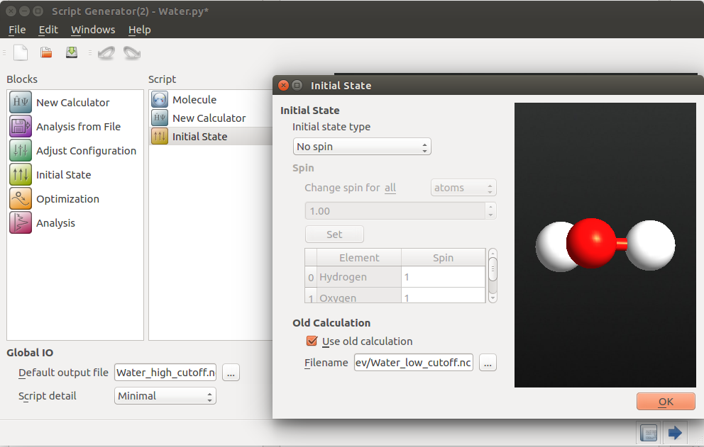
120 Hartree.Add an
 Initial State. Tick the checkbox Use old
calculation, and locate the file
Initial State. Tick the checkbox Use old
calculation, and locate the file water_low_cutoff.hdf5.
This inserts an initial_state variable to setCalculator(), as
mentioned above. Send the script to the Editor  by the
Send To icon at the lower right corner. You will find the
lines in the script. Send it to the Job Manager and run
the calculation.
by the
Send To icon at the lower right corner. You will find the
lines in the script. Send it to the Job Manager and run
the calculation.
You will find that the low accuracy calculation takes 6 self-consistent iterations to converge and the high accuracy calculation takes only a single iteration. If you run the high-accuracy calculation without initialization, it also needs 6 iterations. In this example, as the system is very small, there is not any time save by using this method, due to overhead from initialization etc. But for a realistic system, the high accuracy calculation could be much more time consuming than the low accuracy ones, saving time overall by using this method. We can save a lot of computational time by reducing the number of high accuracy iterations using this strategy.
Note
The first calculation also takes some time and the efficiency of this method varies strongly from case to case. It is only effective if the result from the first calculation is good enough to reduce the number of iterations in the second calculation significantly.
Looping over parameters
Usually, there are numerical parameters which you do not initially know how to choose optimally, that is, the values of parameters which gives a desired balance between calculation time and accuracy. This applies to parameters like k-point sampling and mesh cut-off. Besides using some reasonable physical insight to get a rough idea, a more reliable way is to try different values and see how the results change. This can often be done on a small testing system, and the results can then be applied to a real and larger system of interest.
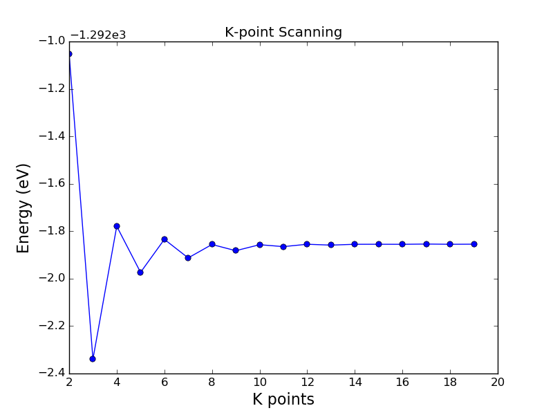
The script kpoint_looping.py checks how many k-points are needed to get a good value
for the total energy of a gold crystal. When doing parameter scanning, it is a
good idea to lower the tolerance of the self-consistent loop, which increases
the accuracy of the solution. In this script we set it two orders of magnitude
lower than default.
Running this script, you will get the following plot, from where you find that a sampling of 12 or 13 k-points along each axis is sufficient for good total energies for gold (valid for this specific combination of basis set, etc).
If you compare to the same calculation without any initial state, i.e. if each calculation is started from neutral atoms, the number of self-consistent iterations is typically more than two times larger, especially when the number of k-points is large (i.e. the most time-consuming parts of the script); thus the benefit of using an initial state in this type of loop is very obvious.
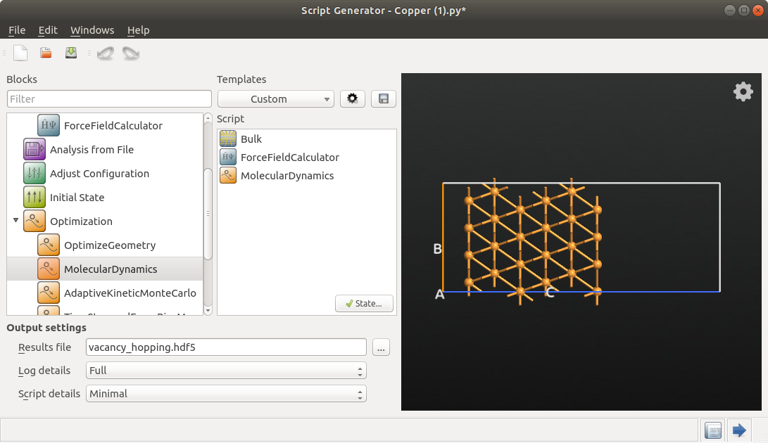
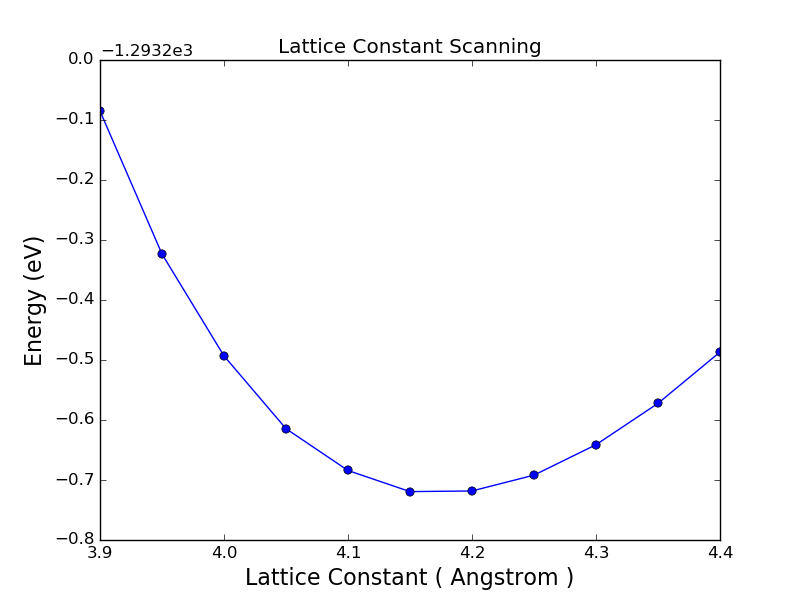
Another very common task is to loop over a variable, like a lattice constant,
to find the lowest total energy for a configuration. This script lattice_const_looping.py is
for finding the equilibrium lattice constant of gold.
Note
To optimize the unit cell size for a system like this, it is often more efficient to use the OptimizeGeometry method in ATK, which can optimize th lattice parameter(s) using an efficient algorithm. The calculation above is still meaningful, however, since it also gives an idea of the error we make by having a non-optimized cell. Furthermore, the values can be used to compute the bulk modulus if you do a more proper 3rd degree polynomial fitting.
In these examples the results are not saved. If you want to do some further processing, like compute the band structure for each configuration and compare those, add such statements inside the loop and store the results in a HDF5 file.
The result of fitting the parabola is a =4.17 Å; if we use GGA instead of LDA ,the value changes to 4.19 Å, i.e. in both cases about 2-3% above the experimental value of 4.08 Å. It is not expected that DFT always gives the experimental value, so this is not an error. A more relevant comparison is, for instance, what a corresponding high-accuracy plane-wave calculation gives, and these typically also overestimate the lattice constant of gold by 1-3% [1].
Stepping up in bias
In the tutorial of Molecular Device, the I-V curve is obtained by climbing in bias using the converged previous state as the initial state.
Special example: anti-parallel spin in MTJs
This strategy has also been used in the magnetic tunnel junction (MTJ) calculation, where it is used initialize a calculation with a new spin configuration compared to the original calculation. This allows you to converge the calculation with a simpler spin-state and use that as a starting point. ATK will rescale the converged density matrix into an initial density matrix for the new calculation according to the distribution of spin up and spin down as given by the initial spin setting of the new calculation.
References