Uniaxial and Biaxial Stress in Silicon
Introduction
In this tutorial you will learn how to use QuantumATK to study the electronic properties of silicon under uniaxial and biaxial stress.
In particular, you will learn how to use the Target Stress option for a geometry optimization (Optimize Geometry) to apply a specific stress to a crystal.
Then you will calculate and analyze the electronic band structure and effective masses in the strained system.
An important aspect of this tutorial is the symmetry of your crystal after the stress is applied. You will have to pay particular attention to this point, and to this end you will find the Brillouin Zone Viewer plugin very useful.
Uniaxial Stress
Set up the Calculation
In the Builder, import a silicon fcc bulk structure from the database and send it to the Script Generator.
Add a
New Calculator:use the default LDA exchange-correlation potential and select a 9x9x9 k-point sampling;
set the density mesh cut-off to 150 Hartree to have a better description of the silicon electronic structure.
Add
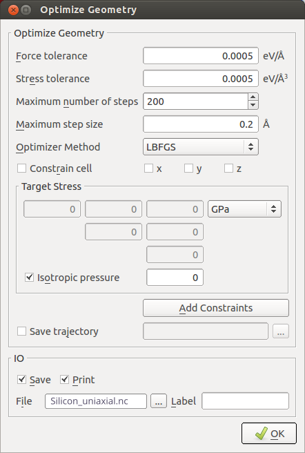
OptimizeGeometryand set these parameters in order to perform a full optimization of the bulk structure:set force and stress tolerances to 0.0005 eV/Å and 0.0005 eV/Å3;
uncheck the
Constrain cellbut keep the target stress at zero.
Add
Bandstructureanalysis:choose 201 points per segment;
choose the L, G, X path.
Add
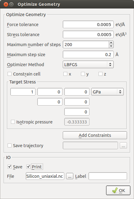
OptimizeGeometryand set these parameters in order to apply a uniaxial stress:set force and stress tolerances to 0.0005 eV/Å and 0.0005 eV/Å3;
uncheck
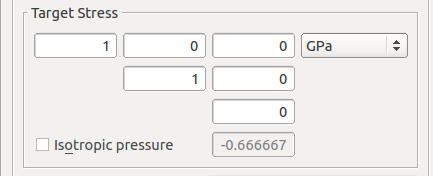
Constrain cell;uncheck
Isotropic Pressureand add a target stress of 1 GPa for the \(x\) component of the stress tensor.
Note
The definition of target stress (
target_stress) is:if a single value \(p\) is given, it will be interpreted as an external pressure value from which the internal target stress tensor is calculated as \(\sigma = \begin{pmatrix} -p & 0 & 0 \\ 0 & -p & 0 \\ 0 & 0 & -p \end{pmatrix}\);
if a target stress tensor is given, it will be interpreted as the internal stress of the system, meaning that a negative entry on the diagonal will result in a compression in the corresponding direction and vice versa. Note that the stress tensor is symmetric, so it’s only necessary to define the upper triangle.
Pay attention to the fact that the sign convention is different in these two cases!
Add
Bandstructureanalysis:choose 201 points per segment;
choose the L, G, X path.
Note
If a target stress tensor is given, the BravaisLattice of the configuration is automatically converted into a UnitCell, to enable changes in the shape of the cell.
As described below, the high symmetry points of the Brillouin zone will change, since the cell will no longer be fcc after the stress is applied. However, at this point in the setup, the symmetry of the new cell is not known, so you will have to modify the symmetry points by hand in the Python script.
Send the script to the Editor and locate the last
Bandstructureanalysis block. Replace X by B in the route; see the next section for a detailed explanation on the modified Brillouin zone.1# ------------------------------------------------------------- 2# Bandstructure 3# ------------------------------------------------------------- 4bandstructure = Bandstructure( 5 configuration=bulk_configuration, 6 route=['L', 'G', 'B'], 7 points_per_segment=201, 8 bands_above_fermi_level=All 9 ) 10nlsave('Silicon_uniaxial.nc', bandstructure)
You can download the full script here:
Silicon_uniaxial.py.Save and send the script to the Job Manager to run the calculations, which should take less than a minute.
Symmetry Considerations
Before analyzing the electronic structure of strained silicon you will need to understand how the Brillouin zone and the notation of high symmetry points are dealt with by QuantumATK.
From the LabFloor drag and drop the optimized structure (gID000) and the strained structure (gID002) to the Builder.
Plot the Brillouin zone of each structure with the Bulk Tools->Brillouin Zone Viewer…:
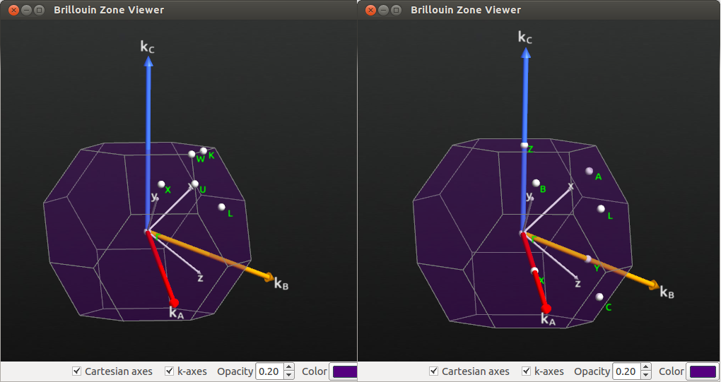
Fig. 103 Brillouin zone for fcc bulk silicon when FaceCenteredCubic Bravais lattice is used (left).
When the Bravais lattice is changed to UnitCell type, the notation for high symmetry points is changed according to the figure (right).
The high symmetry points in the UnitCell representation of the strained fcc crystal are related to the fcc symmetry points as follows:
A, B, C all correspond to the X point in the unstrained fcc Brillouin zone.
By increasing the stress you can see that B and C are still degenerate, but A is not degenerate with B and C. This is logical in the tetragonal symmetry.
The L point is still called L, and degenerate with X, Y, Z in the UnitCell notation.
The symmetry of the crystal is actually, as expected, tetragonal (space group 141) after the uniaxial stress is applied, which can be verified by activating the strained crystal on the stash and using Bulk Tools->Crystal Symmetry Information, and clicking Detect. On inspection of the lattice parameters, you see that, again as expected, all 3 lattice vectors are elongated in the X axis, and contracted in Y and Z (elastic response, Poisson effect), due to the uniaxial deformation.

Analyze the Results
Electronic Band Structure
Now plot the band structure of the optimized cell and the uniaxial stressed cell.
From the LabFloor select the calculated Bandstructure object and plot them with the Bandstructure Analyzer plugin.
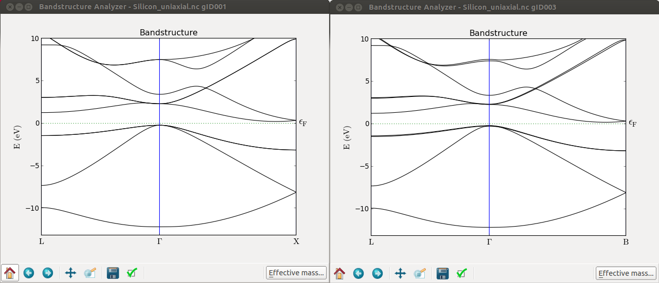
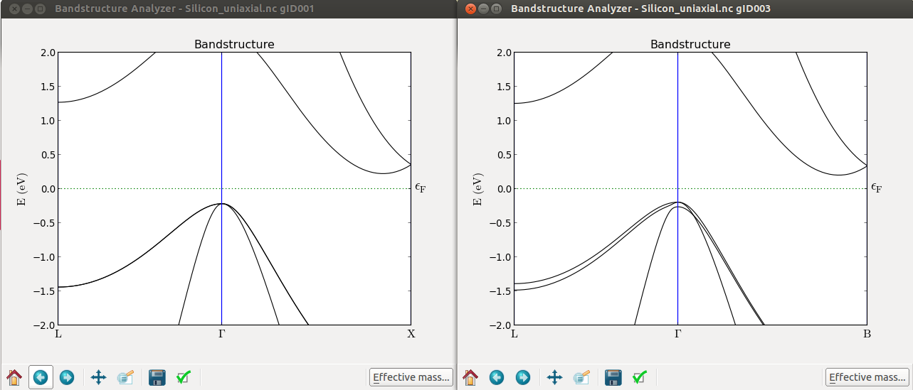
From these plots you can immediately see that, at Gamma, the top of the valence band splits. It is however, more interesting to see that the \(\Delta\) valley is not degenerate anymore. To see this effect more clearly you can calculate the band structure along the A-G-B path.
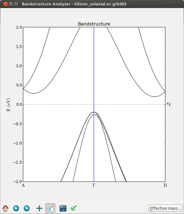
By further inspecting the band structure, you can conclude the following about uniaxially strained Si:
L remains degenerate
The 6-fold \(\Delta\) valleys split into 2+4
The absolute values of the band gaps are however not correct in this simulation, since the LDA exchange-correlation functional was used for simplicity.
Effective Masses
It is also very interesting to consider the effects of strain on the effective mass.
From the band structure plot of the strained structure, click on the Effective Mass button.
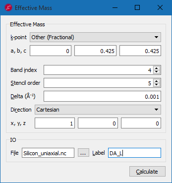
Following the example in the figure above calculate the effective masses for the \(\Delta\) valleys, band index 4, along different directions:
Longitudinal mass at \(\Delta_A\): fractional coordinate [0, 0.425, 0.425], along the [1,0,0] cartesian direction;
Transverse mass (1) at \(\Delta_A\): fractional coordinate [0, 0.425, 0.425], along the [0,1,0] cartesian direction;
Transverse mass (2) at \(\Delta_A\): fractional coordinate [0, 0.425, 0.425], along the [0,0,1] cartesian direction;
Longitudinal mass at \(\Delta_B\): fractional coordinate [0.425, 0, 0.425], along the [0,1,0] cartesian direction;
Transverse mass (1) at \(\Delta_B\): fractional coordinate [0.425, 0, 0.425], along the [1,0,0] cartesian direction;
Transverse mass (2) at \(\Delta_B\): fractional coordinate [0.425, 0, 0.425], along the [0,0,1] cartesian direction;
You will find the following results:
Longitudinal mass at \(\Delta_A\) (2-fold degenerate): 0.91
Transverse masses at \(\Delta_A\): 0.185 (no split)
Longitudinal mass at \(\Delta_B\) (4-fold degenerate): 0.898
Transverse masses at \(\Delta_B\): 0.188 and 0.186
So, while all longitudinal and transverse masses are very close to the original \(\Delta\) valley masses (0.903 and 0.186, which you can compute from unstrained crystal), you see splittings due to the broken symmetry.
For a more detailed explanation on the calculation of silicon effective masses please refer to the tutorial Effective mass of electrons in silicon.
As an exercise, you are encouraged to study the masses at the L point, and investigate possible symmetry breakings.
Biaxial Stress
Take the optimized (unstrained) silicon structure, send it to the Scripter and set New Calculator, OptimizeGeometry, and Bandstructure as you did in the previous section.
To apply a biaxial stress, set the xx and yy components in the stress tensor to 1 GPa in the Target Stress field in the Optimize Geometry dialog.
Before running the calculation, send the script to the Editor and modify the Brillouin zone path to L, G, B as described above and run the calculation.
Also in this case the cubic lattice distorted is to a tetragonal symmetry. To see that clearly, drag and drop the optimized stressed structure to the Builder and apply the supercell transformation as indicated in the figure below.
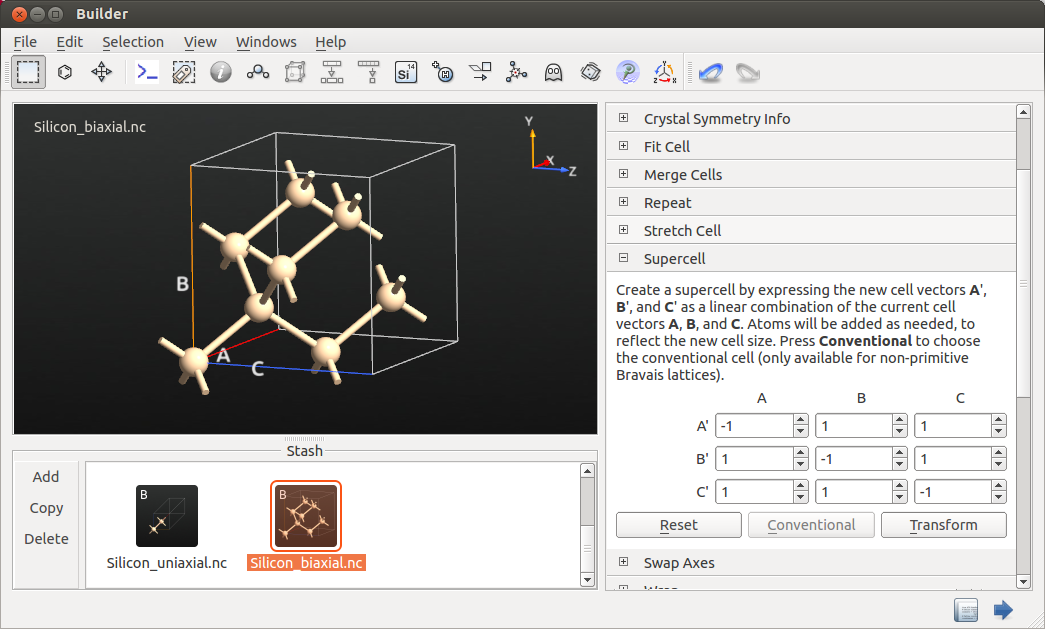
From Bulk Tools->Lattice Parameters you can see the distorted lattice parameters of 5.44 Å and 5.38 Å. Thus, effectively the biaxial stress is equivalent to a uniaxial stress along the [001] direction, with opposite sign.