How to calculate reaction barriers using the Nudged Elastic Band (NEB) method
Version: U-2022.12
In this tutorial you will learn how to calculate reaction barriers for a reaction with well-defined initial and final states. As an example, we will use the diffusion of a single platinum ad-atom on a Pt(100) surface, but the methodology can be used in any situation where you can define an initial and final state of the system, connected by movement of one or more atoms.
Specifically, in this tutorial you will:
create the Pt(100) surface with a Pt ad-atom;
create a high-quality initial NEB path and run the NEB calculation;
analyze the results and compare with the literature.
In order to have more details about the parameters used to construct and optimize the NEB object, you can check the NudgedElasticBand and OptimizeNudgedElasticBand pages in the manual.
Note
The NEB method employed in this tutorial requires the a priori knowledge of the initial and final configurations of the reaction, which is often a non-trivial task. However, other powerful methods, such as the Adaptive Kinetic Monte Carlo (AKMC) tool, allow study of reaction barriers in a system from just a user-defined initial state, as shown in Adaptive Kinetic Monte Carlo Simulation of Pt on Pt(100).
Create the initial and final states for the NEB
In this section you will set-up the structure of a Pt ad-atom on Pt(100), which will be used as the initial and final configurations in the NEB calculations. First, you will relax bulk platinum with the chosen calculator to ensure the Pt(100) slab does not have an inherent strain.
Relax bulk platinum
Open QuantumATK and create a new project (f.ex. Pt_Pt100_NEB). Relax bulk platinum with a ForceFieldCalculator using the EAM_Pt_2004 parameter set and default optimization parameters. This simulation runs in a few seconds. If needed, you can download the workflow for this calculation here: Pt_bulk_workflow.hdf5.
Tip
Tutorial on geometry optimization: Geometry optimization: CO/Pd(100)
Create the initial state - a Pt(100) surface with a Pt ad-atom
Use the relaxed platinum bulk configuration to construct a \(5\times5\) (100) slab with a thickness of 4 layers, using the Surface (cleave) tool in the Builder.
Tip
A guide to the Surface (cleave) tool: Cleave tool guide
In the Stash, right-click with the mouse on the newly created Pt_bulk (100) object and select Duplicate. Then, right-click on the newly created Pt_bulk (100) (1) object and select Rename to change its name to initial.
Click on the
 icon to open the Camera panel, and orient the system along the XY direction.
While holding down the
CTRLbutton on your keyboard, use the left mouse button to select a square of four Pt atoms of the Pt(100) topmost layer. Then add an extra atom in between them by clicking on the icon.
icon.Select the new Pt atom, and click on in the Panel plugins on the right-hand side of the screen. Define the translation vector as 1.6 in the z-direction to move the atom about 1.6 \(\text{Å}\) above the surface plane.
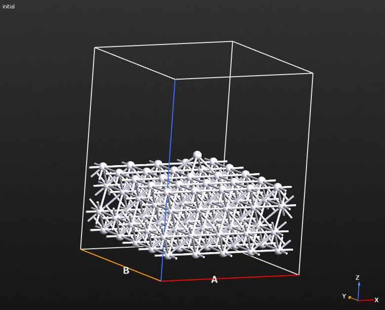
The structure you have just obtained for a Pt ad-atom on Pt(100) will be used as the initial configuration for the NEB calculations performed in this tutorial.
Create the final configuration for the direct jump process
In this section, you will set up the final configuration for the most direct diffusion process possible for a Pt ad-atom on Pt(100), in which the ad-atom jumps directly between neighboring four-fold hollow sites of the Pt(100) surface.
In the Stash, duplicate the initial configuration and change its name to final_jump
Select the final_jump configuration in the Stash, select the Pt ad-atom and click .
In the Translate Panel, translate the Pt ad-atom 2.77195 Å in the x or y-direction.
In this way, you have obtained the final configuration for the NEB calculation of the direct jump diffusion process.

Relax the initial and final configurations
To ensure we get the best possible initial guess for the reaction path between the initial and final states, we need to relax them before constructing it. Use the same calculator as before to relax the two slabs with an ad-atom to a tolerance of 0.01 eV/Å, and using FIXED atom constraints on the bottom two layers of the slab. You can use this workflow to do it: relax_initial_and_final_WF.hdf5
Set up and run the NEB calculations
Construct the NEB path
In the Builder, click on and drag and drop the relaxed initial and final configurations into the left and right panels.
In the Nudged Elastic Band panel, set the Interpolation to Image dependent Pair Potential. Click Create to create an object in the Stash named NEB: initial final, containing the initial and final configurations as well as the interpolated configurations along the reaction path.

Note
The image dependent pair potential (IDPP) [1] implemented in QuantumATK provides high quality initial guesses for the NEB reaction path compared to the more commonly employed linear interpolation method. For complex reaction paths, the improvement in terms of number of required iterations and speed can be substantial.
Run the NEB calculations
Click on the
 icon and send the NEB: initial final configuration to the Workflow Builder.
In the Workflow Builder, change the output Filename at the bottom of the middle panel to
NEB_Pt-jump.hdf5.Add the following blocks to the Build panel by double clicking on the corresponding icons in the QuantumATK tab in the right-hand panel:
Under Calculators:
 Set ForceFieldCalculator
Under Optimization and Dynamics:
 OptimizeNudgedElasticBand
Double-click on the
Set ForceFieldCalculator block and select the EAM_Pt_2004 parameter set again.Double-click on the
OptimizeNudgedElasticBand block, set the Force tolerance to 0.01 eV/\(Å\) and set FIXED constraints on the bottom two layers.Send the workflow to the Job Manager as a script and save the script as
NEB_Pt-jump.py. This script runs in a few seconds, it can run locally.
You should now have a workflow identical to this one: NEB_jump_workflow.hdf5
Analyze the results
Once you have run the NEB calculations for the direct jump diffusion process, many new objects should appear in the Data View section of QuantumATK NanoLab. There is a NudgedElasticBand object for each step in the optimization. They are stored in the file you defined before, here called NEB_Pt-jump.hdf5.

Select the last NEB trajectory, i.e. the one with the highest number, which contains the optimized NEB path for the direct jump process. Then, double-click on it to open it in the Movie Tool.
On the left, the Movie Tool shows the energy of each image, referenced to the energy of the first image. On the right is the corresponding atomic configuration of each image. You can now see the energy barrier for this diffusion process as the highest point in the plot on the left, and see the corresponding transition state configuration on the right by moving the cursor so the vertical gray line is at the transition state.

Fig. 120 Calculated reaction path for the direct jump diffusion process.
Note
As it can be seen in the tutorial at Adaptive Kinetic Monte Carlo Simulation of Pt on Pt(100), the AKMC method finds this path, among others, without any a priori knowledge of the potential energy surface of the system.
Summary
Throughout this tutorial, you have used a ForceField calculator and the NanoLab graphical user interface to set up, simulate and analyze the direct jump diffusion path for a Pt ad-atom on a Pt(100) surface. You can also repeat this tutorial with DFT by replacing the Set ForceFieldCalculator blocks with Set LCAOCalculator blocks, to compare directly with the DFT results reported in the literature [2].