In this tutorial, you will learn how to use QuantumATK NanoLab GUI to
Set-up optical property simulations of dielectric constant, refractive index, IR spectra, absorption spectra, etc. for SiO2 (quartz) using Density Functional Theory (DFT).
Analyze obtained results.
All the workflow, input and output files can be found in the Example Project - Y-2026.03 ‣ SiO2-quartz-dielectric-tensor folder.
Setting up an Optical Property Calculation Workflow
QuantumATK can calculate many different optical properties from the DielectricTensor, including both electronic and ionic contributions, such as dielectric constant, refractive index, reflectivity, extinction coefficient, optical absorption coefficient, IR spectra, susceptibility. Follow the step-by-step protocol described below to set up these simulations for SiO2 (quartz) in the Workflow Builder.
Follow the tutorial Geometry Optimization to import the structure of bulk SiO2 (quartz) from NanoLab’s Crystal Database to the Workflow Builder.
Go to the Block Catalog ‣ QuantumATK tab ‣ Analysis category on the right hand panel and drag-and-drop the DielectricTensor block to the middle Workflow Area ‣ Build tab.
Workflow Builder automatically adds-in the Optical Spectrum block (for the electronic part of the dielectric tensor), and then Dynamical Matrix and Born Effective Charge blocks (for the ionic part of the dielectric tensor) to the workflow. You see the warning signs, because the calculators are not yet specified for these blocks (see the next steps).
Go to the Block Catalog ‣ QuantumATK tab ‣ Calculators and Optimization and Dynamics categories on the right hand panel and drag-and-drop the SetForceFieldCalculator and OptimizeGeometry blocks, respectively, to the middle Workflow Area ‣ Build tab, above the DynamicalMatrix block.
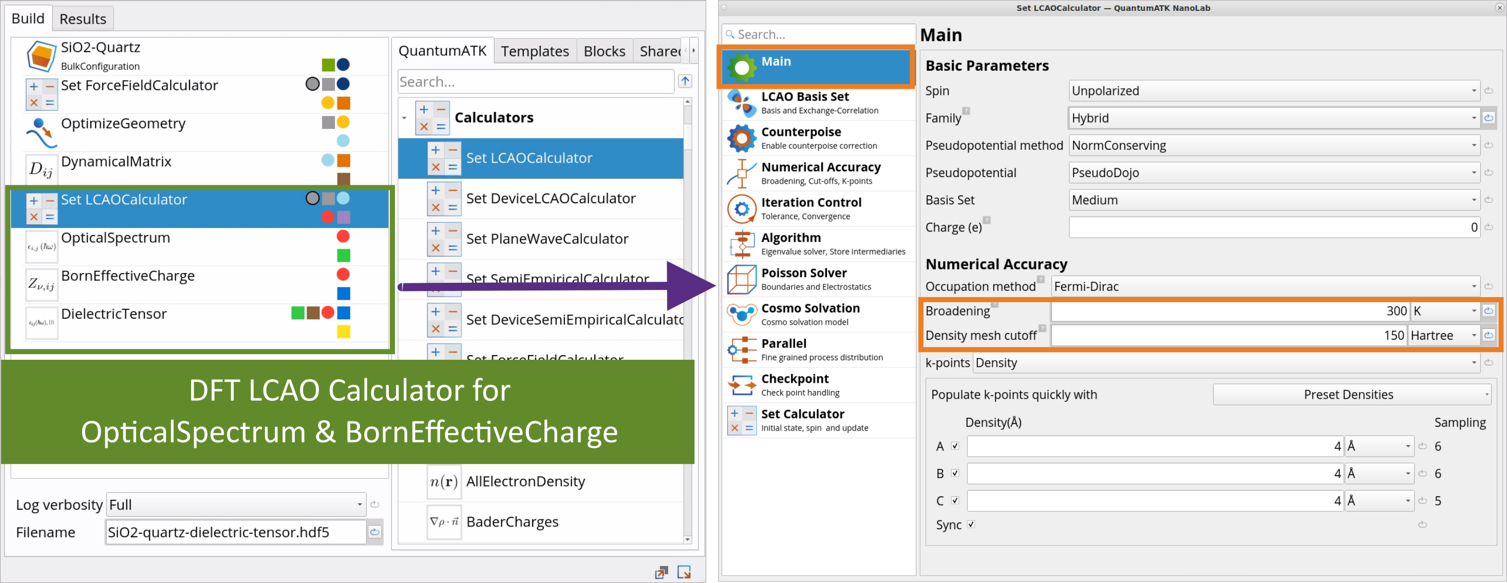
Go to the Block Catalog ‣ QuantumATK tab ‣ Calculators category and drag-and-drop the SetLCAOCalculator block to the middle Workflow Area ‣ Build tab, below the DynamicalMatrix block, to define the DFT LCAOCalculator that will be used for OpticalSpectrum and BornEffectiveCharge simulations. The full workflow for optical property calculations is shown below.
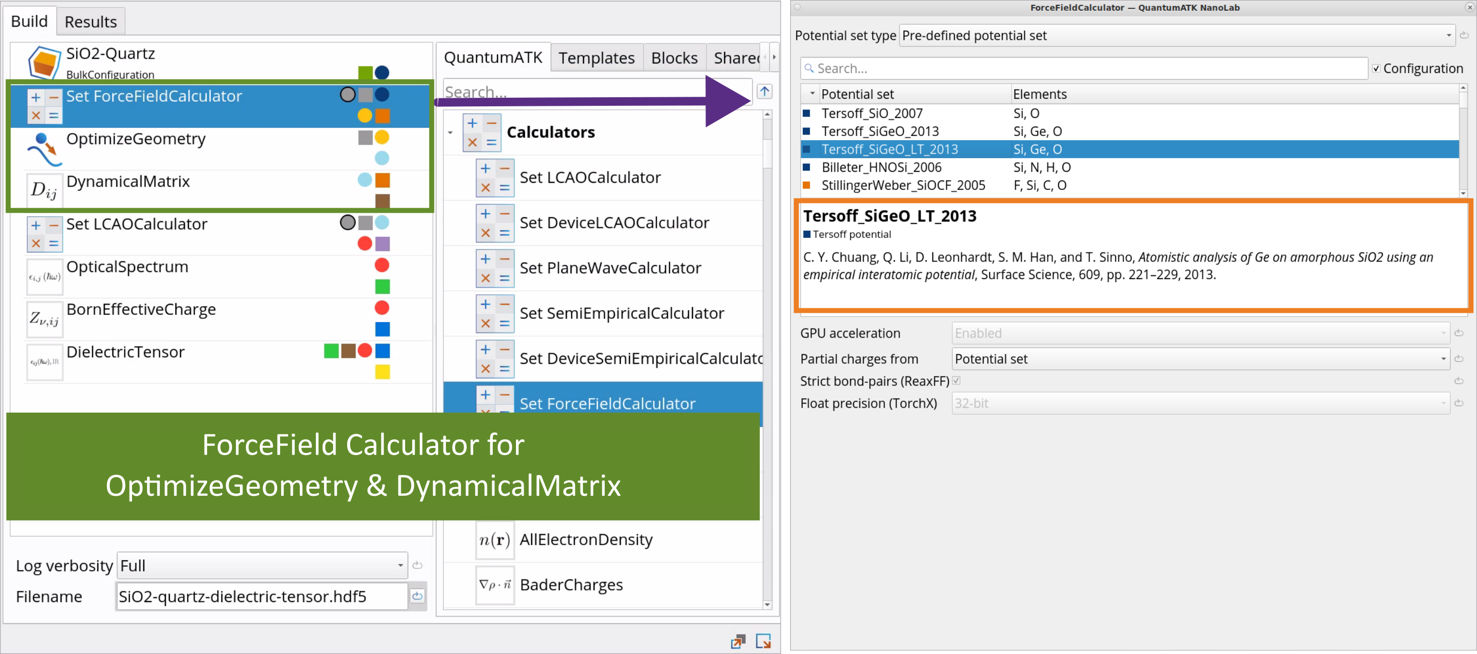
Double-click on the SetForceFieldCalculator block and choose a Tersoff_SiGeO_LT_2013 Force Field for OptimizeGeometry and DynamicalMatrix calculations. It is important to use the same calculator for both geometry optimization and dynamical matrix simulations.
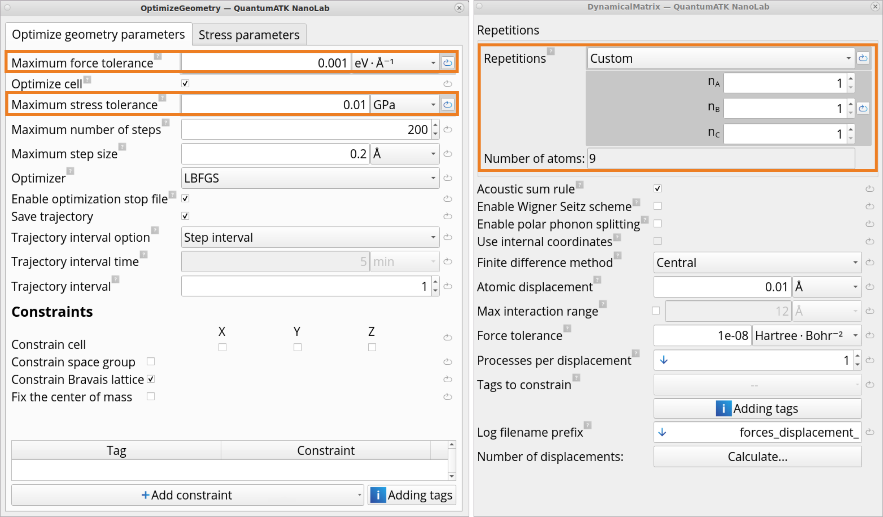
Double-click on the OptimizeGeometry block and set a tighter than default force (0.001) and stress (0.01) tolerances, as it is important to have a very well converged geometry for the subsequent dynamical matrix simulations.
Double-click on the DynamicalMatrix block and change the Repetitions to Custom: 1, 1, 1, as you need to include vibrations only at the Γ point and do not need a repeated super cell. This makes the calculation computationally much cheaper (and manageable with DFT if it is chosen instead of Force Fields) as now you need to calculate displacements for 9 atoms instead of 2205 atoms in the default 7 x 7 x 5 repetition.
Double-click on the SetLCAOCalculator block and make the following edits:
Under the Main tab, increase the Density Mesh Cutoff from the default 125 Ha to 150 Ha as this is necessary for obtaining accurate and converged Born effective charges and thus optical properties, in particular the dielectric constant’s ionic part. Change the numerical accuracy parameter Broadening from 1000 K to 300 K (recommended for semiconductor materials).
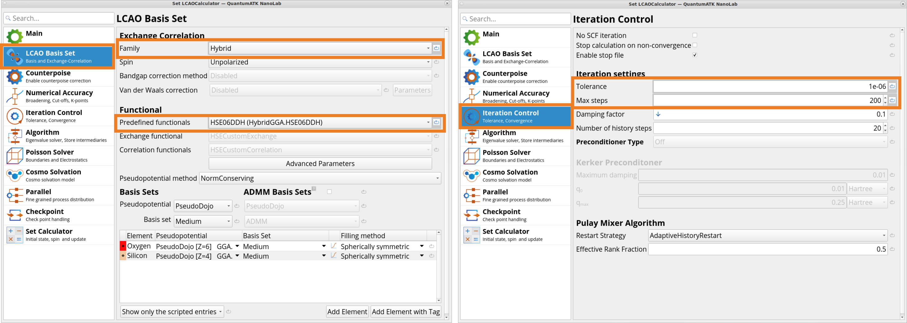
Under the LCAO Basis Set tab, change the Exchange CorrelationFamily from the default GGA to Hybrid and for the Predefined functional choose HSE06DDH (Hybrid.GGA.HSEO6DDH). Here, we will use a dielectric dependent hybrid functional HSE06-DDH (DDHCustomExchangeCorrelation) as it provides accurate electronic structure for SiO2 (quartz), as shown in the Tutorial Band Structure, Projected Density of States and Effective Mass Calculations, which is important for optical properties.
Under the Iteration Control tab, set a tighter than default SCF convergence tolerance (1e-06 vs. 1e-04), which is also crucial for calculating accurate and converged Born effective charges. In addition, increase the Max steps for SCF from the default 100 to 200 so the SCF cycle converges even if it needs more steps due to the tighter tolerance.
Tip
SetLCAOCalculator block sets medium k-point sampling and medium basis set by default, typically providing good accuracy results with modest computational resources. It is recommended to check the convergence of your results with these parameters.
SetLCAOCalculator block uses a default Fermi-Dirac Occupation Method with 1000 K Broadening, which generally works reasonably well across various systems. Another setting may be more appropriate for your system, and you can adjust these settings according to the recommendations in Occupation Methods for semiconductor, insulator, metal, and molecule systems.
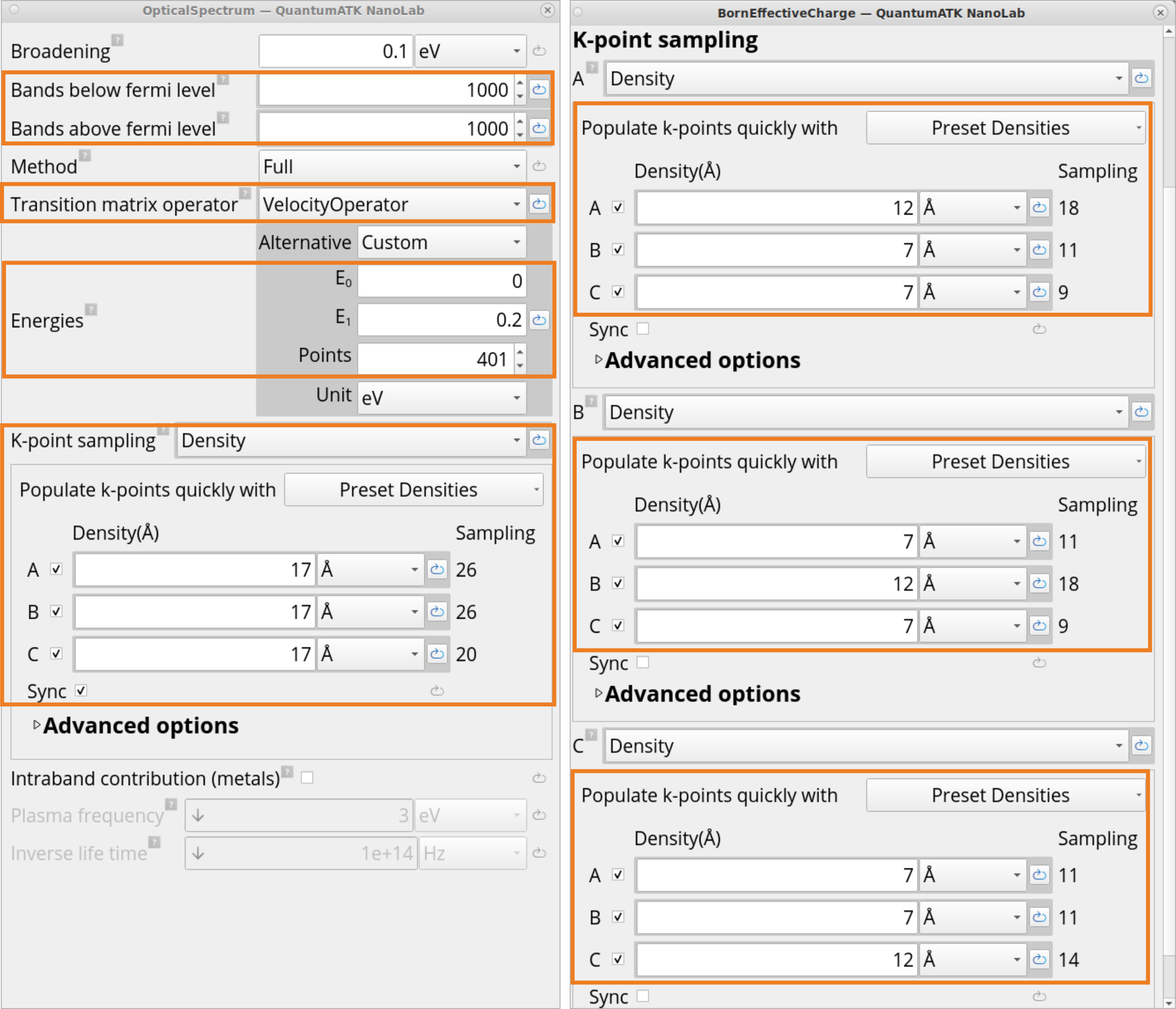
In the OpticalSpectrum block, change the following settings to calculate OpticalSpectrum accurately:
Change the default number of Bands below/above Fermi level to arbitrary 1000 (as the default 4 is too few for SiO2 (quartz)).
For the Transition matrix operator method, select the VelocityOperator (which is also the default method for the DFT-LCAO calculator with Norm Conserving PPs), as it gives a more accurate optical spectrum compared to the MomentumOperator method.
Select the energy range 0 – 0.2 eV and change to 401 points for finer sampling. This will ensure a high-resolution IR spectrum, which typically features many narrow and closely spaced peaks corresponding to different vibrational modes.
For the k-point sampling, choose Density and click on Preset Densities to increase the k-point density from medium to higher, i.e., 17Å x 17Å x 17Å. It is important to have a large k-point sampling for properties that depend on the conduction band minimum, for example, dielectric constant and electron transport properties.
Tip
When calculating absorption spectra, it is recommended to select a wider energy range and use default (more coarse) sampling. This is because an absorption spectrum typically covers a broader range of wavelengths and can include various types of transitions, often resulting in broader peaks compared to those in IR spectra.
In the BornEffectiveCharge block, for the k-point sampling, choose Density and click on Preset Densities to increase the k-point density from medium to high, i.e., A: 12Å x 7Å x 7Å, B: 7Å x 12Å x 7Å, C: 7Å x 7Å x 12Å.
The DielectricTensor block has no adjustable paramaters. It takes in calculated DynamicalMatrix, OpticalSpectrum and BornEffectiveCharges in previous steps to compute the DielectricTensor.
Change the Workflow name in the the Workflow Stash and Filename as needed (e.g., SiO2-quartz-dielectric-tensor.hdf5).
Click on the Send content to other tools button and choose Jobs as a script to send the workflow to the Jobs tool to submit this job on a local machine or a remote cluster.
This also generates a Python script SiO2-quartz-dielectric-tensor.py, based on this workflow. It can be opened and edited with the Editor tool and then sent to the Jobs tool.
The BornEffectiveCharge tensor is defined as the derivative of the polarization with respect to the atomic coordinate and is used for DielectricTensor calculation.
Once the calculation has finished, we are ready to analyze the results.
Go to the Data View tool.
In the Data Sources, select the file SiO2-quartz-dielectric-tensor.hdf5 and then double-click on the DielectricTensor_0 object in the Data View window to open it with the Dielectric Tensor Analyzer.
Tip
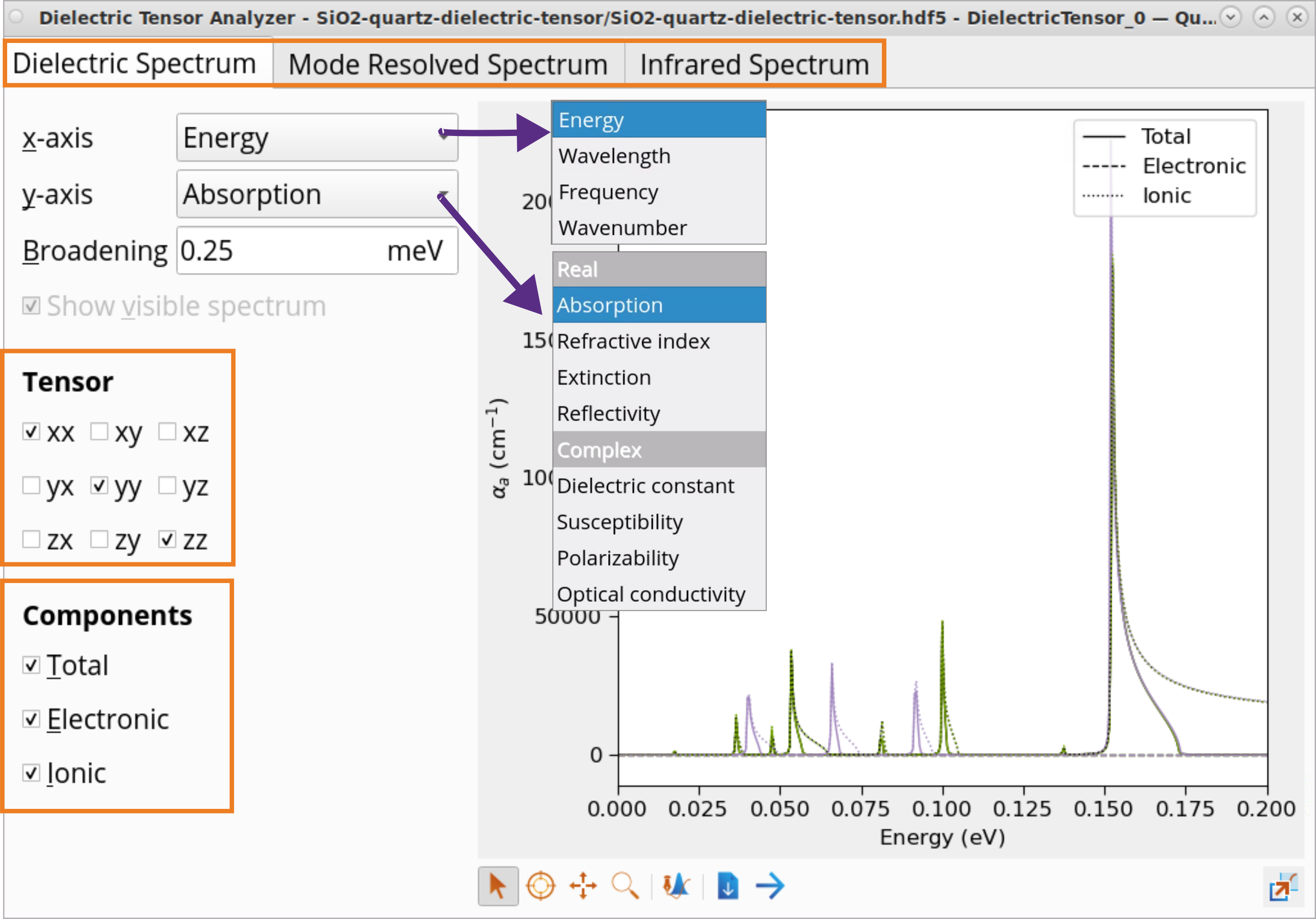
The Dielectric Tensor Analyzer can plot a range of optical properties. In the Dielectric Spectrum panel, click on y-axis to see the list: Absorption, Refractive index, Extinction, Reflectivity, Dielectric constant, Suscpetibility, Polarizability, Optical conductivity as a function of Energy, Wavelength, Frequency or Wavenumber (x-axis).
Plot Mode resolved spectrum and Infrared Spectrum.
Plot differet tensor components (xx, yy, zz) and total, electronic and ionic contributions to the optical properties.
To plot and analyze the dielectric constant:
Select the Dielectric constant (y-axis) as a function of Energy (x-axis).
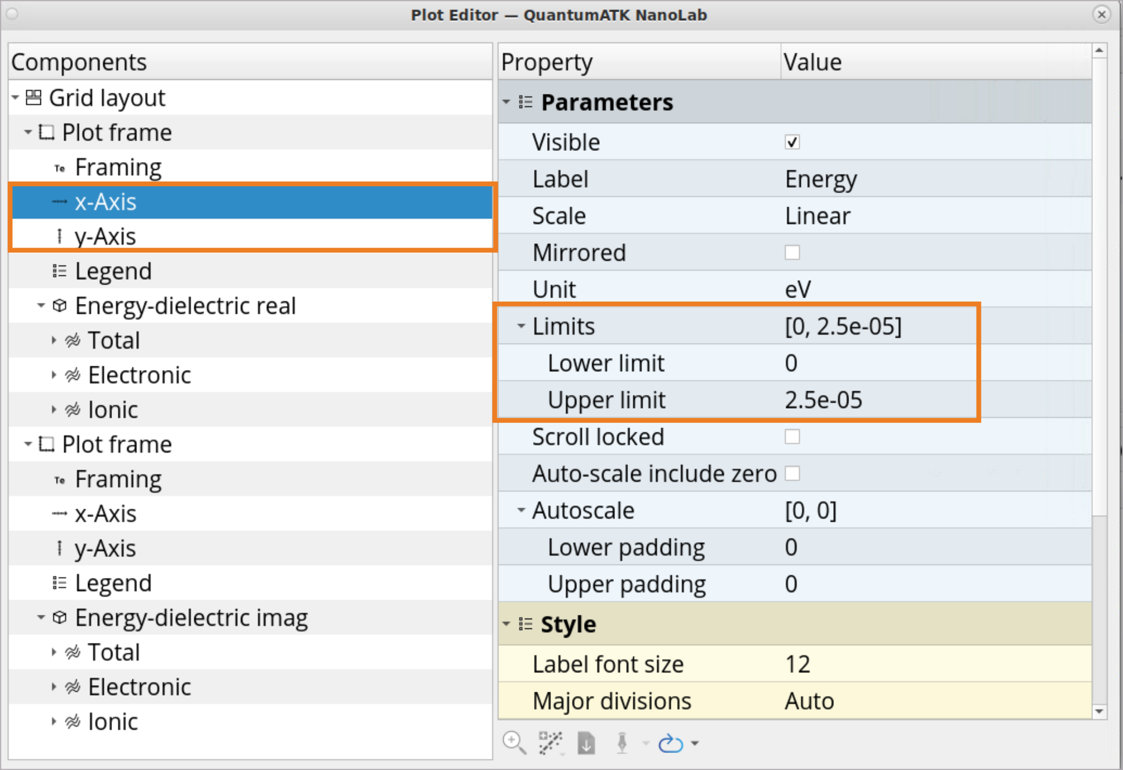
Click on the x axis and then on the Plot editor button.
Adjust the Lower limit and Upper limit to x and y axes to zoom into the \(Re[ε]\) at \(E\) = 0 eV to determine the static dielectric constant, \(ε_0\). For the x axis, select a range from 0 to 2.5e-05, and for the y axis, select a range from 0 to 10.
Use the Inspect tool to examine dielectric constant values for SiO2 (quartz):
total: \(ε_{0_{xx/yy}}\) = 3.72 and \(ε_{0_{zz}}\) = 3.92
ionic contribution: \(ε_{ion_{xx/yy}}\) = 1.61 and \(ε_{ion_{zz}}\) = 1.81
Note
Ionic contribution to the SiO2 (quartz) static dielectric constant is significant and cannot be neglected.
The calculated dielectric constant, \(ε_0\), and symmetry break are in a reasonably good agreement with the experimental results at a room temperature: \(ε_{0_{⊥}}\) = 4.43 and \(ε_{0_{∥}}\) = 4.64, in the directions perpendicular to and along the trigonal axis, respectively [1].
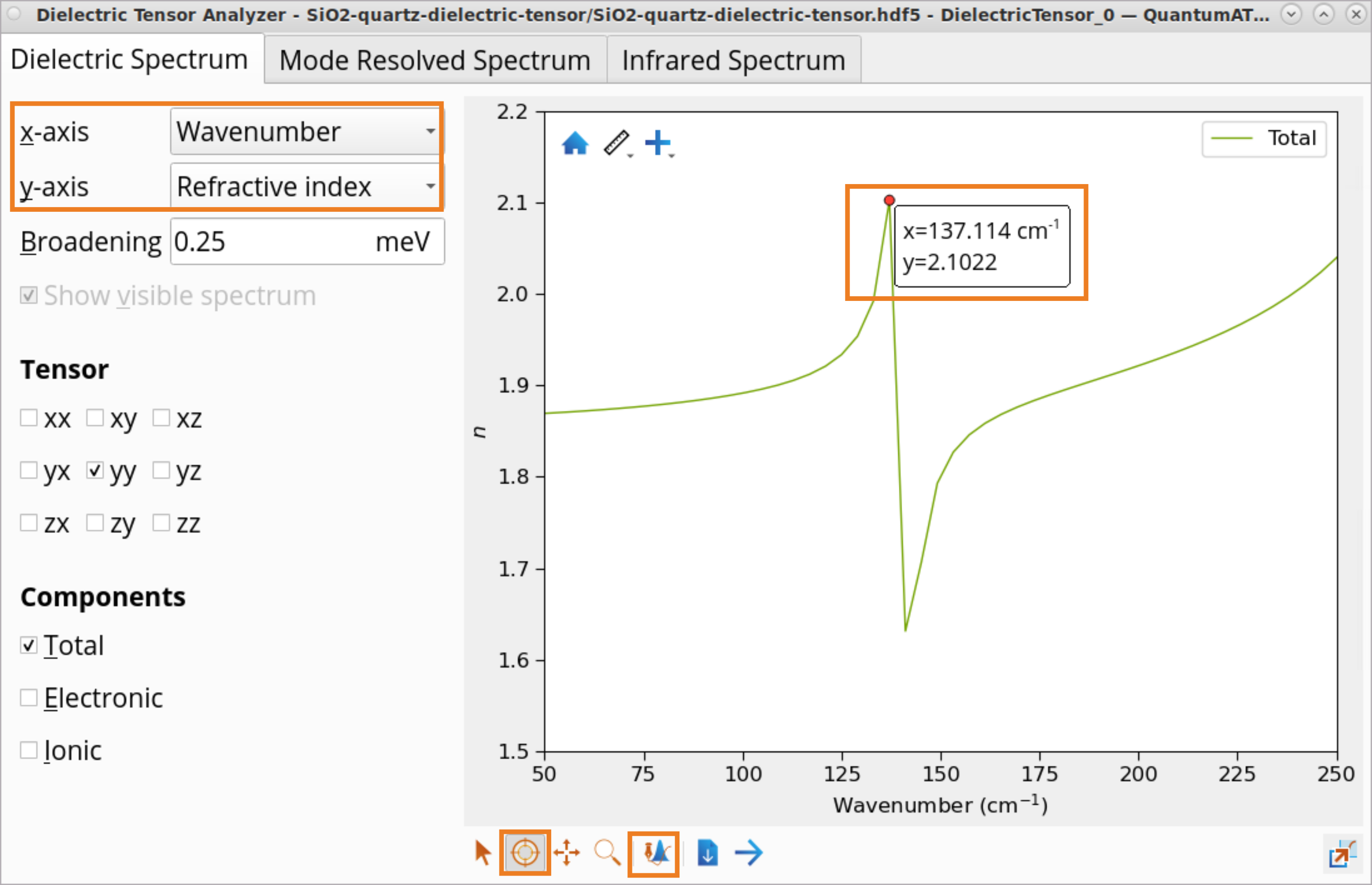
To plot and analyze refractive index:
Select the Refractive index (y-axis) as a function of Wavenumber (x-axis).
Click on the Plot editor to zoom in on the refractive index \(n\) at around 50-250 \(cm^{-1}\).
Use the Inspect tool to examine refractive index values at the peaks: e.g., \(n_{yy}(137cm^{-1})\) = 2.10 and \(n_{yy}(141 cm^{-1})\) = 1.63.
Note
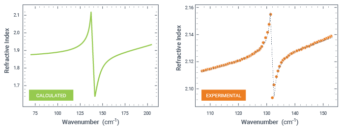
The simulated refractive index at 0 K is in a qualitative agreement with the experimental results at 10 K [2] as shown in the Figure below.
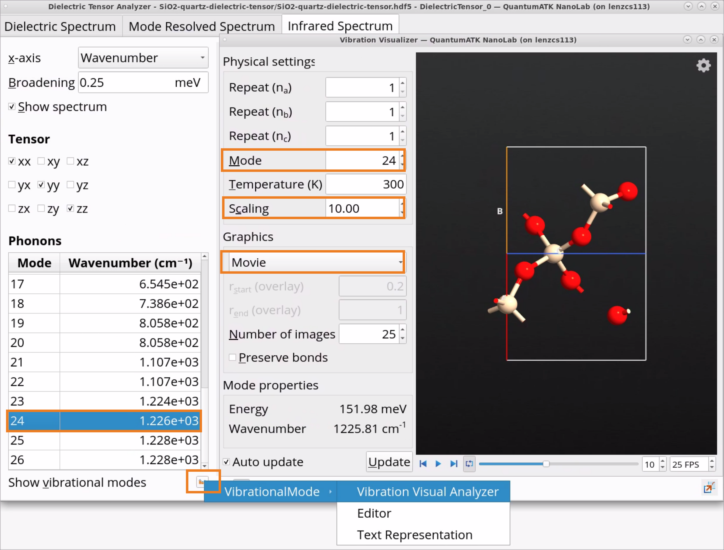
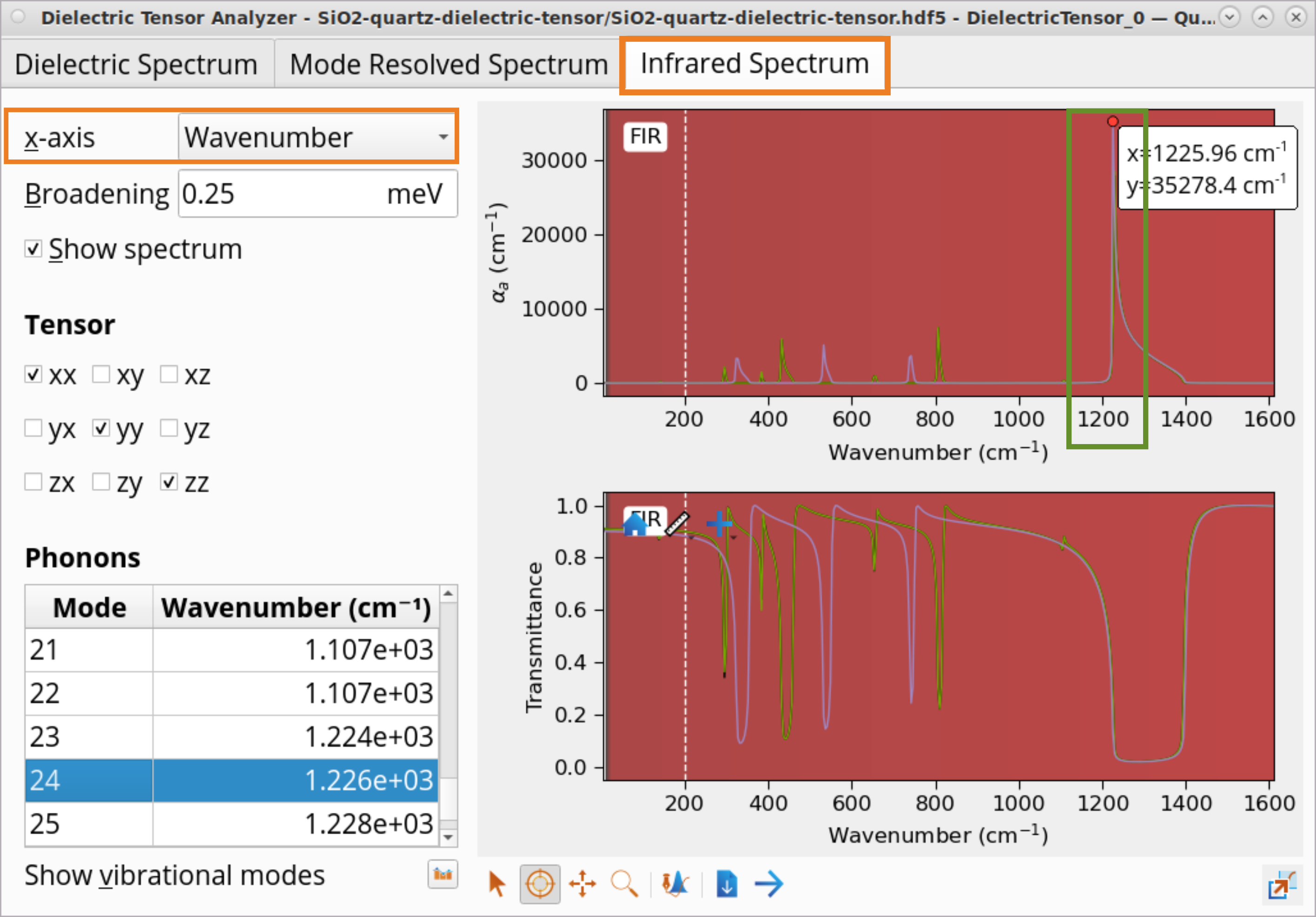
5.Click on the Infrared Spectrum tab to examine the calculated IR spectrum.
Due to the temperature effects and random crystal orientations in the powder, the experimentally measured IR peak is broader than the calculated one for the single crystal direction at 0K.
Click on the Show vibrational modes icon and choose Vibration Visual Analyzer to visualize chosen vibrational modes.
In the Vibration Analyzer, choose a vibrational mode, e.g., 24.
Set Scaling to 10.
Under Graphics, choose Movie to see the actual vibration for mode 24 at 1226 \(cm^{-1}\) corresponding to the highest peak in the IR spectrum.
For polar materials, it is possible to apply polar-phonon (LO-TO) splitting to the vibrational modes beyond the workflow presented here. This effect can be included by adding the optical properties and Born effective charge to the dynamical matrix analysis, and doing so will increase the LO mode vibrational frequency (observable in Raman spectroscopy for instance).

 Workflow Builder.
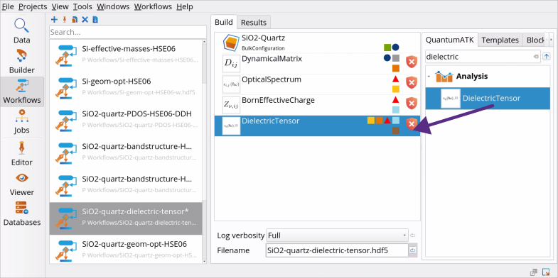
 SetForceFieldCalculator and
  OptimizeGeometry blocks, respectively, to the middle Workflow Area ‣ Build tab, above the DynamicalMatrix block.
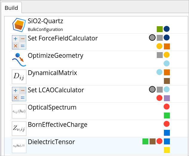
 Send content to other tools button and choose Jobs as a script to send the workflow to the
  Jobs tool to submit this job on a local machine or a remote cluster.
 Editor tool and then sent to the
  Data View tool.
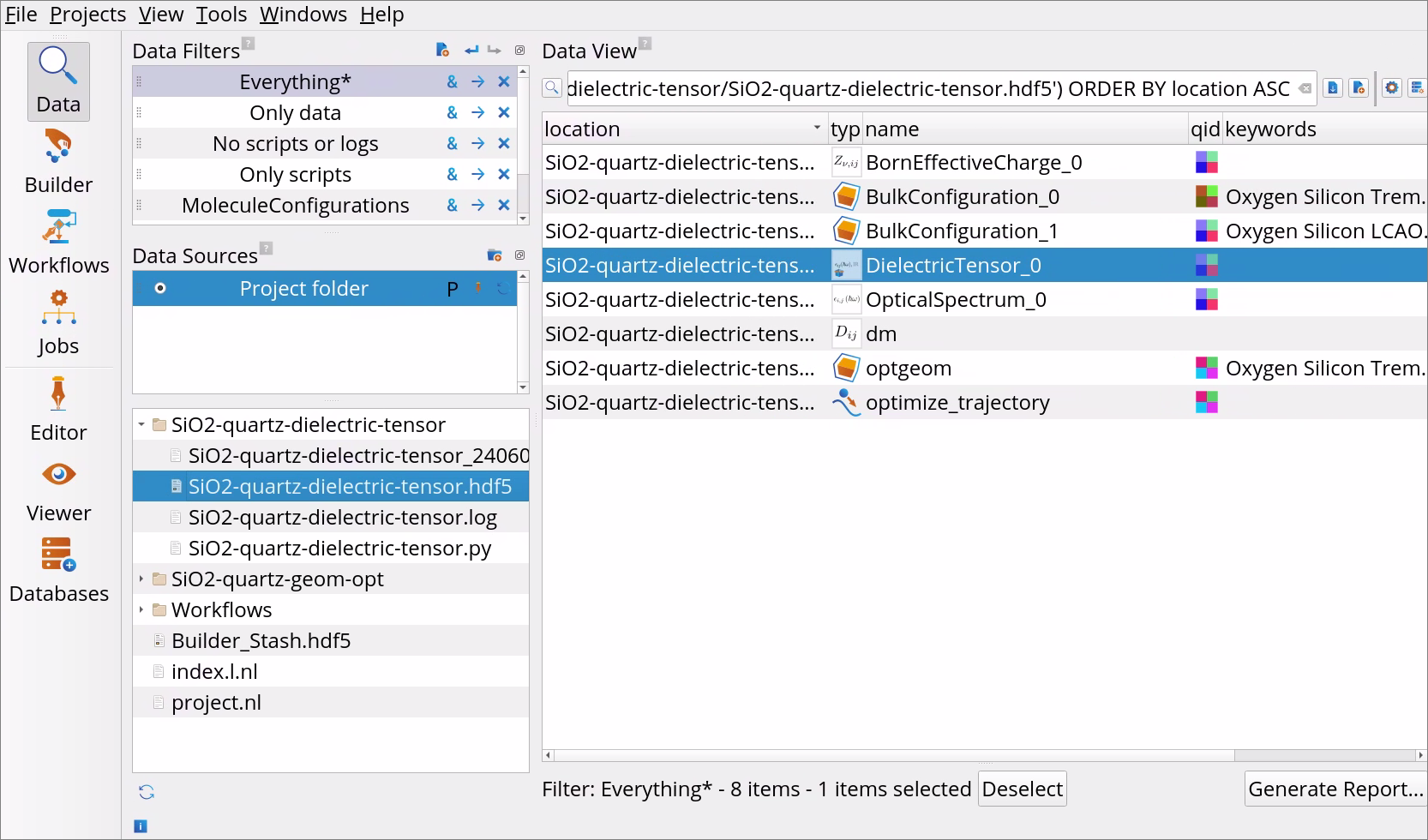
 Plot editor button.
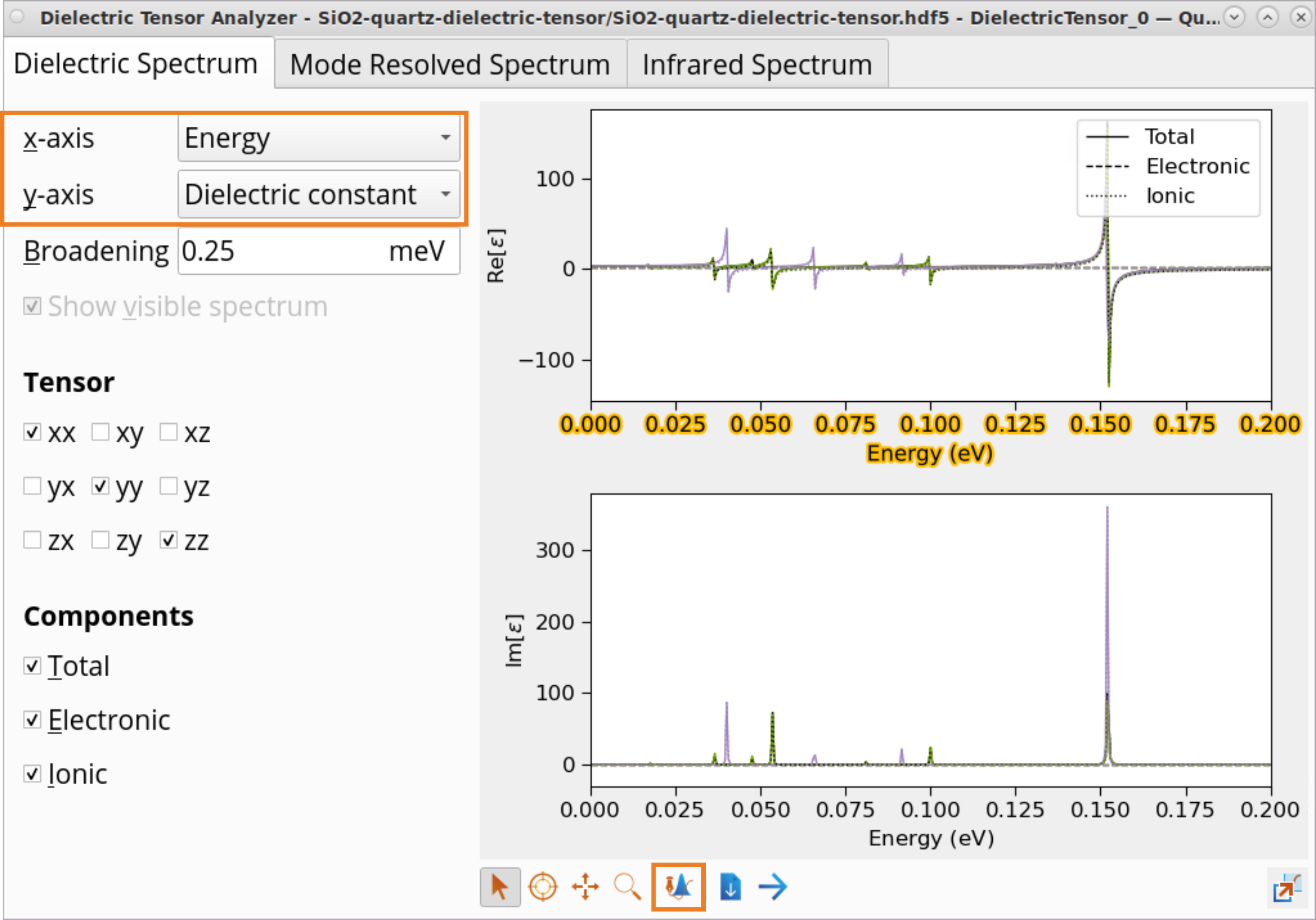
 Inspect tool to examine dielectric constant values for SiO2 (quartz):
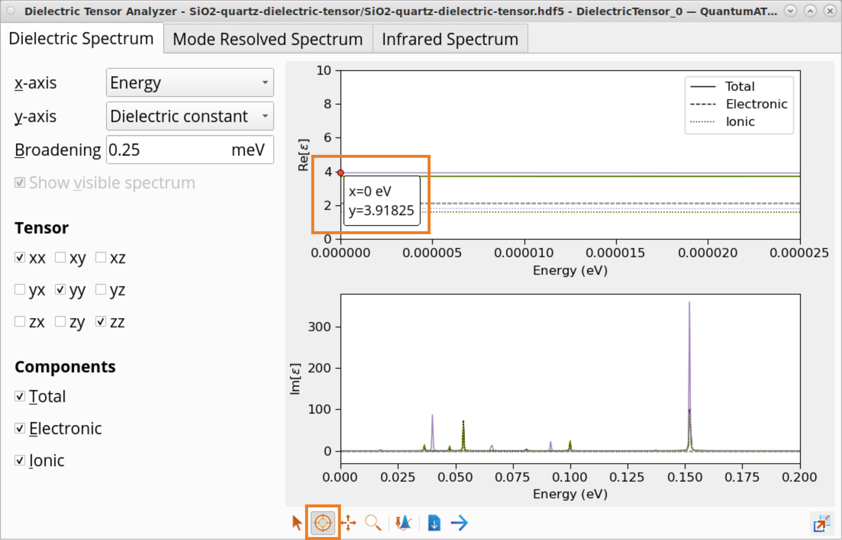
 Show vibrational modes icon and choose Vibration Visual Analyzer to visualize chosen vibrational modes.