Introducing the QuantumATK plane-wave DFT calculator
Version: 2017.0
The ATK-DFT plane-wave calculator was introduced in QuantumATK 2017.0, and this tutorial gives a brief introduction to how to use it. We will look at a simple bulk example to introduce the basic functionalities of this calculator.

Introduction
The central difference between the plane-wave (PW) calculator and the LCAO calculator is that the one-electron eigenstates are expanded in a plane-wave basis set instead of atom-centered basis functions. The plane-wave representation of electronic structure has a long tradition in computational studies of periodic bulk systems, and has the key advantage that the basis set can systematically be improved by simply increasing the number of plane waves included in the calculation (albeit at a significantly increased computational cost). This makes the PW calculator an interesting alternative to the usual LCAO calculator for studies of (not too large) bulk systems, and may also be used as a benchmark in investigations of the accuracy of an LCAO basis set for a specific system.
As an example, we will find the lattice constant and band structure of bulk copper, but first we need to converge the size of the PW basis to make sure our results are accurate.
Warning
Note that in the 2017 version of QuantumATK, the plane-wave calculator is still a beta version, so not all functionality has been implemented, and it has a higher risk of bugs. From QuantumATK O-2018.06 it is a finished product with full functionality.
Converging the PW basis
The number of plane waves included in the PW calculation depends on the plane-wave cutoff energy \(E_\mathrm{cut}\). The accuracy of the PW calculation increases as the number of plane waves increase (larger \(E_\mathrm{cut}\)), but so does also the computational cost. The desired trade-off between computational accuracy and cost must therefore be chosen, and we use a convergence study for this.
To converge the PW basis, we compute some desired property for a range of cut-off energies, here the total energy, in order to investigate how large \(E_\mathrm{cut}\) needs to be in order to get sufficiently accurate results.
To do this, follow these steps:
Open the Builder
 and click on .
Type “copper” to search for pure copper, select it and press the
 button.
Now send the configuration to the Script generator

Add New Calculator
 and Total energy
  objects.
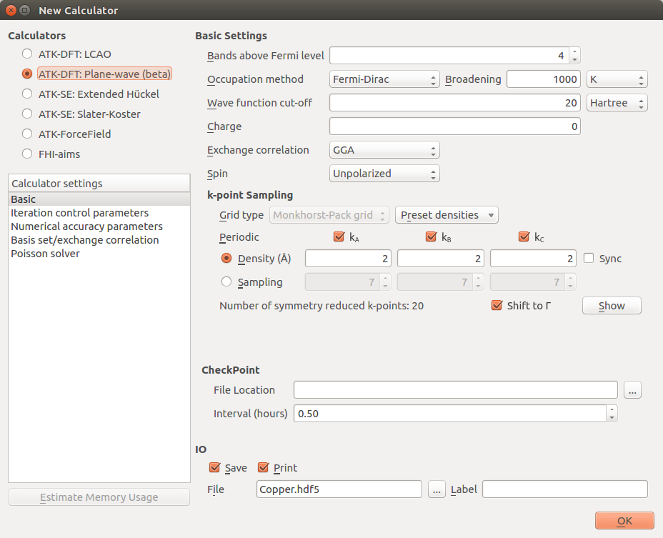
Open the New Calculator and change it to ATK-DFT: Plane-wave (beta).
Your New Calculator window should look like this:
Click Ok and send the script to the Editor
 by using the
  .
.
We now need to create the loop over the PW cutoffs. Insert these lines at the top of the script, after the line specifying the encoding, to calculate the total energy for cutoffs ranging from 10 to 100 Hartree:
e_cut_list = range(20,110,10)*Hartree

for e_cut in e_cut_list:
You also need to indent everything after these lines.
Tip
You can easily indent many lines in the Editor by selecting them, and pressing the Tab key.
Finally, we need to change the values for the cutoffs to the variable that is being used in the for-loop. Find the line where the density mesh cutoff is defined, it should be line 37 now, and replace it with the following:
density_mesh_cutoff=e_cut*4,
Find the line where the calculator is defined, and insert wave_function_cutoff=e_cut, to make the calculator look like this:
    calculator = PlaneWaveCalculator(
        wave_function_cutoff=e_cut,
        numerical_accuracy_parameters=numerical_accuracy_parameters,
        )
Note
The default mesh cutoff is 4 times the PW cutoff, which ensures that there is no loss of accuracy from this and no unnecessary computational overhead.
Your script should now look like this: e-cut-conv.py, and you can run it. It should take no more than half an hour on a modern laptop, and significantly less if MPI parallelization is used.
Tip
We plan to introduce a new feature in 2018 which allows you to set up this process from the Script Generator.
In some cases where you want to redo a previous calculation, but with a higher PW cutoff, it can be beneficial to restart the calculation. It is slightly more complicated to set up the script this way, but in our case it will make the calculation run a little faster, reducing the time required by about a factor of 2. An example of this script can be seen here: restart-e-cut-conv.py.
After running the script, we can now plot the total energy of the system vs. the PW cutoff. You can use this simple script to plot the data: plot-e-cut-conv.py. It will generate two plots. One for all values of the cutoff, and one where the first values are omitted, to allow for a clearer picture in the region of convergence. The second plot should look like this:
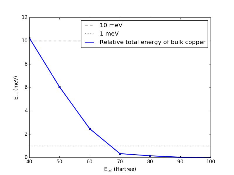
It shows that the total energy has converged to within 10 meV per atom with a cutoff of 50 Hartree, while 70 Hartree is required to converge the energy within 1 meV of the chosen reference calculated with a cutoff of 100 Hartree. The choice of reference and convergence criteria is a decision for the user, and should be based on the needed accuracy, balanced against the computational cost. In this case, we are mostly interested in fast calculations, and so we choose a cutoff of 50 Hartree.
Tip
The required cutoff depends strongly on both the element and the specific pseudopotential, so you should always test convergence when using a new pseudopotential.
Calculating properties
Now that we have found the PW cutoff needed for satisfactory accuracy, we can calculate some properties for bulk Cu. We will do a simple calculation of the lattice constant and the bandstructure. Go back to the Script Generator window.
Add OptimizeGeometry
 and Bandstructure objects.
Move the objects around to ensure that the
is just after the .Open the New Calculator object and change the cutoff to the 50 Hartree we found previously.
Open the OptimizeGeometry object and un-check Constrain Lattice Vectors
Send the script to the Job Manager to run it. It should look like this:
cu-bulk.py
Running the script took about 10 minutes using 8 MPI processes on an 8-core machine, so anything up to a couple of hours is possible if run on a laptop.
Tip
The ATK-PW calculator uses symmetry to reduce the number of k-points that must be calculated, and it parallelizes over the reduced k-points. In order to get the most efficient parallelization, you should check this reduced number in the Script Generator, and use a number of MPI processes which is as close to a divisor of this number as possible.
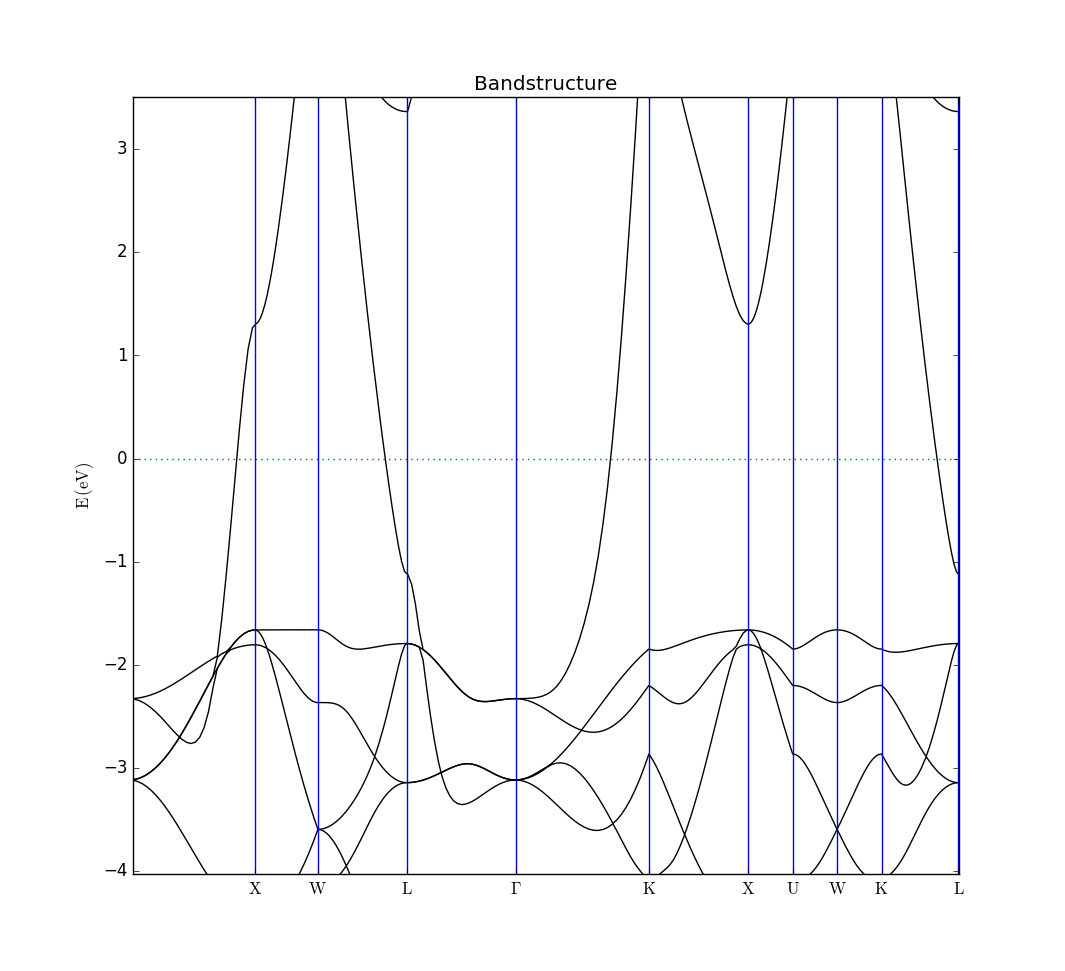
You can now inspect the log-file Copper.log and the data-file Copper.hdf5 and verify that we have found a lattice constant for copper of 3.660650 Å after stress and force optimization, a total energy of -4968.92 eV and the following bandstructure, if zoomed in on a range around the Fermi level.
Other analysis objects
Not all QuantumATK analysis objects support the PW calculator in QuantumATK 2017.0, as it is still in beta. However, the Script Generator is aware of this fact, and will cross out any unsupported analysis objects, and will omit them when the actual script is generated and sent to the Editor or the Job Manager. If the script is created manually, QuantumATK will give an error message when it encounters an analysis object which does not support the plane-wave calculator.