Molecular Dynamics Simulations for Generating Amorphous Structures
Molecular Dynamics Simulations for Generating Amorphous Structures
Version: Y-2026.03
In this tutorial, you will learn how to use QuantumATK NanoLab GUI to
Prepare an initial structure for amorphous SiO2 using Amorphous Prebuilder based on Packmol.
Set-up Molecular Dynamics (MD) melt-quench and subsequent MD equilibration simulations to generate a final equilibrated amorphous SiO2 structure using classical Force Fields.
Analyze obtained results, such as radial and angular distribution functions, RDF and ADF, to verify the quality of the generated amorphous SiO2 structure.
Set-up a geometry optimization simulation for amorphous SiO2 in order to obtain a 0 K structure, representing the most stable configuration. This optimized structure can serve as a reference state for further calculations of electronic properties, phonons and other thermodynamic properties.
All the workflow, input and output files can be found in the Example Project - Y-2026.03 ‣ Am-SiO2-MD folder.
To create a workflow for generating an initial amorphous structure, performing MolecularDynamics melt-quench and equilibration simulations in the Workflow Builder, follow the step-by-step protocol described below. Here, we will use a classical Force Field Tersoff_SiO_2007.
Go to the Block Catalog ‣ Templates tab ‣ Molecular Dynamics category on the right hand panel and drag-and-drop the Constant Density Melt Quench (Force Field) template to the middle Workflow Area ‣ Build tab. You see the warning signs, because the Force Field calculator and the initial amorphous structure are not yet specified for these blocks (see the next steps).
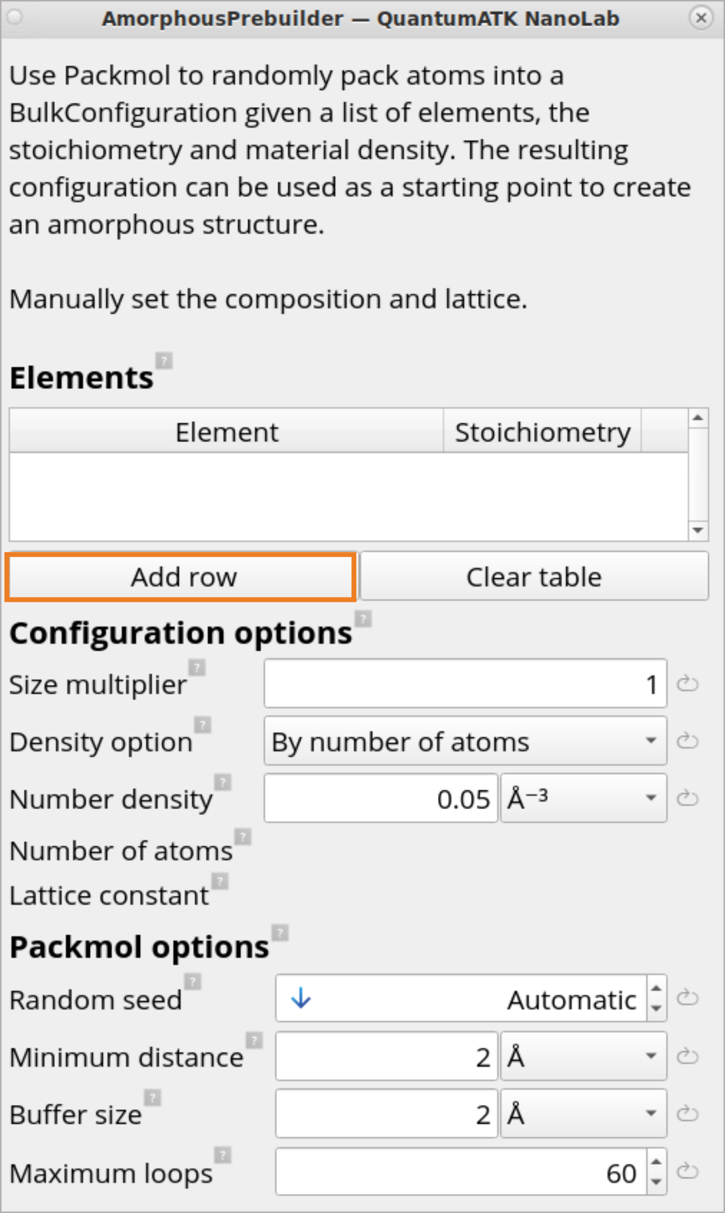
Click on the AmorphousPrebuilder block to set up a generation of an initial amorphous structure from selected elements on-the-fly. It will use Packmol to randomly pack atoms into a bulk configuration given a list of elements stoichiometry and material density.
Click on Add row button.
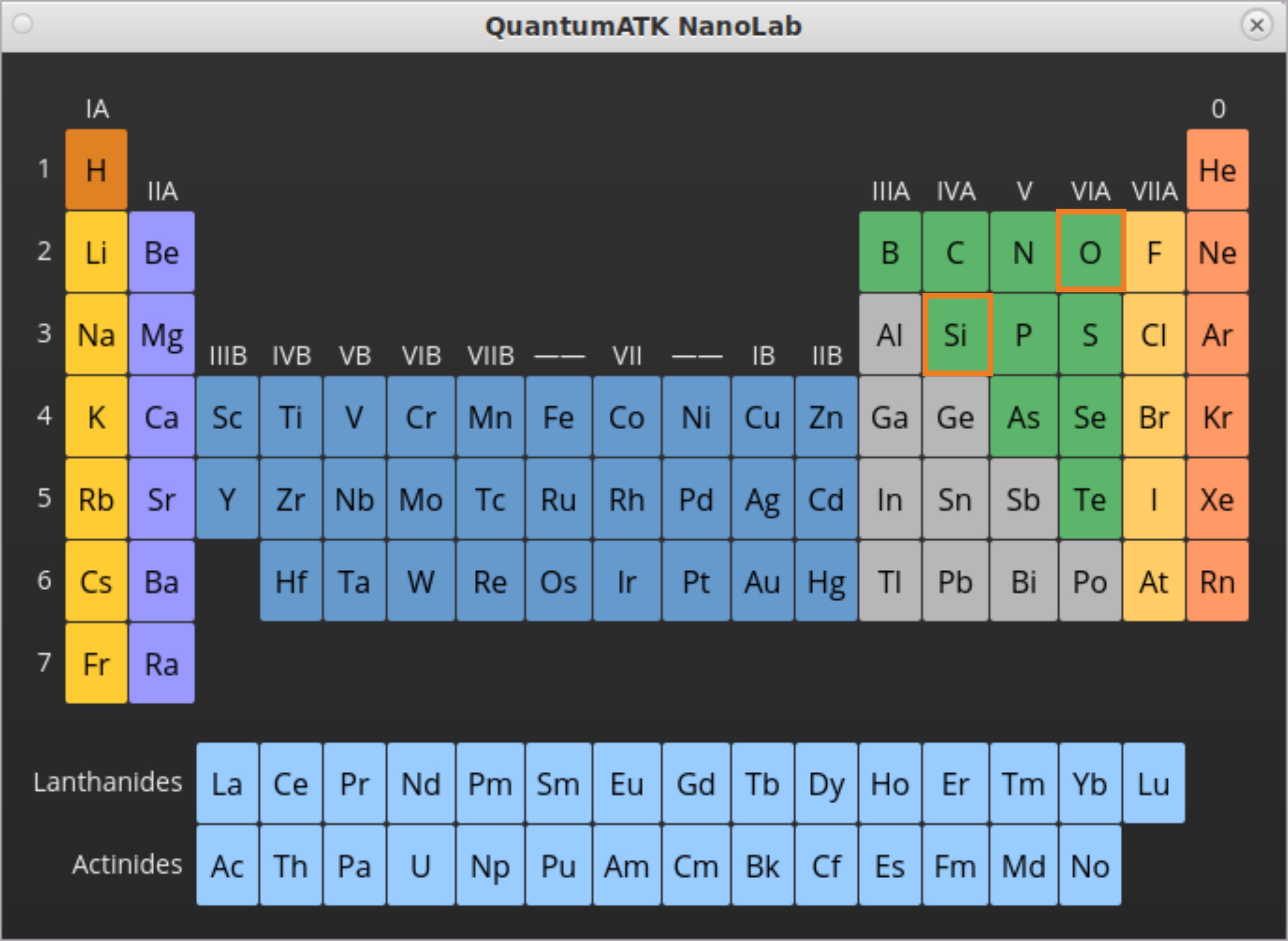
In the opened Periodic Table window, click on Si to add it to the AmorphousPrebuilder.
Repeat the steps to add O to the AmorphousPrebuilder.
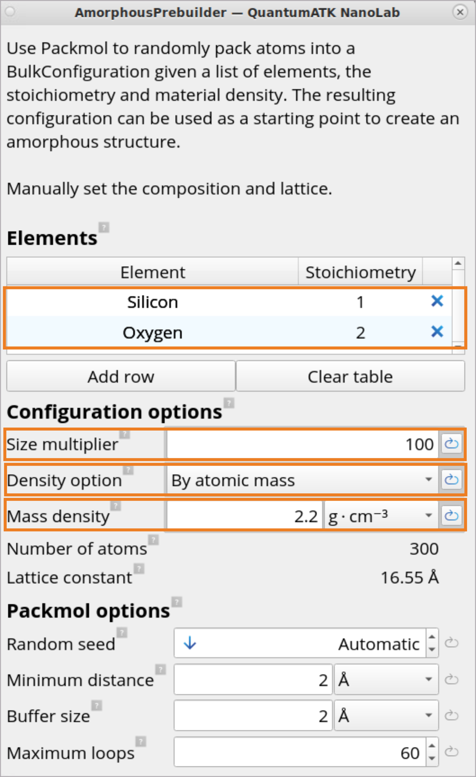
Set Stoichiometry1 to Si and 2 to O.
Set Size multiplier to 100 to generate an initial amorphous cell with 100 Si and 200 O atoms.
For Density option, choose By atomic mass and specify 2.2\(g ⋅ cm^{-3}\)Mass density for the amorphous SiO2 structure. This will automatically determine the Lattice constant of 16.55 Å.
The generated initial amorphous structure will automatically be passed into the 2nd part of the simulation workflow, which includes melt-quench and equilibration MD simulations.
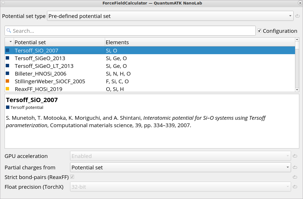
Click on the Set ForceFieldCalculator block and choose Tersoff_SiO_2007 Classical Force Field.
Tip
For systems for which there is no conventional Force Field available or the quality is not good, we recommend to use Machine Learned Force Fields (ML FFs). Consider:
Using pre-trained custom Moment Tensor Potentials (MTPs) for a specific target system and application or pre-trained universal MACE or M3GNet Neural Network (NN) potentials. The list of available ML FFs can be found in the SetMachineLearnedForceFieldCalculator block.
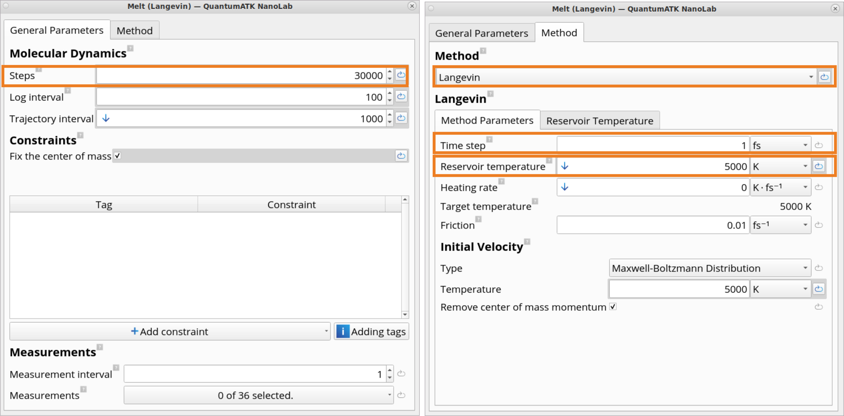
4. Click on the Melt (Langevin) block, which contains settings for the Langevin type MD simulations at high (i.e., 5000 K) temperature to melt the structure.
In this example, you will run 30 000 MD steps with a time step of 1 fs, resulting in a total MD melt simulation time of 30 ps. Use the settings set by the template.
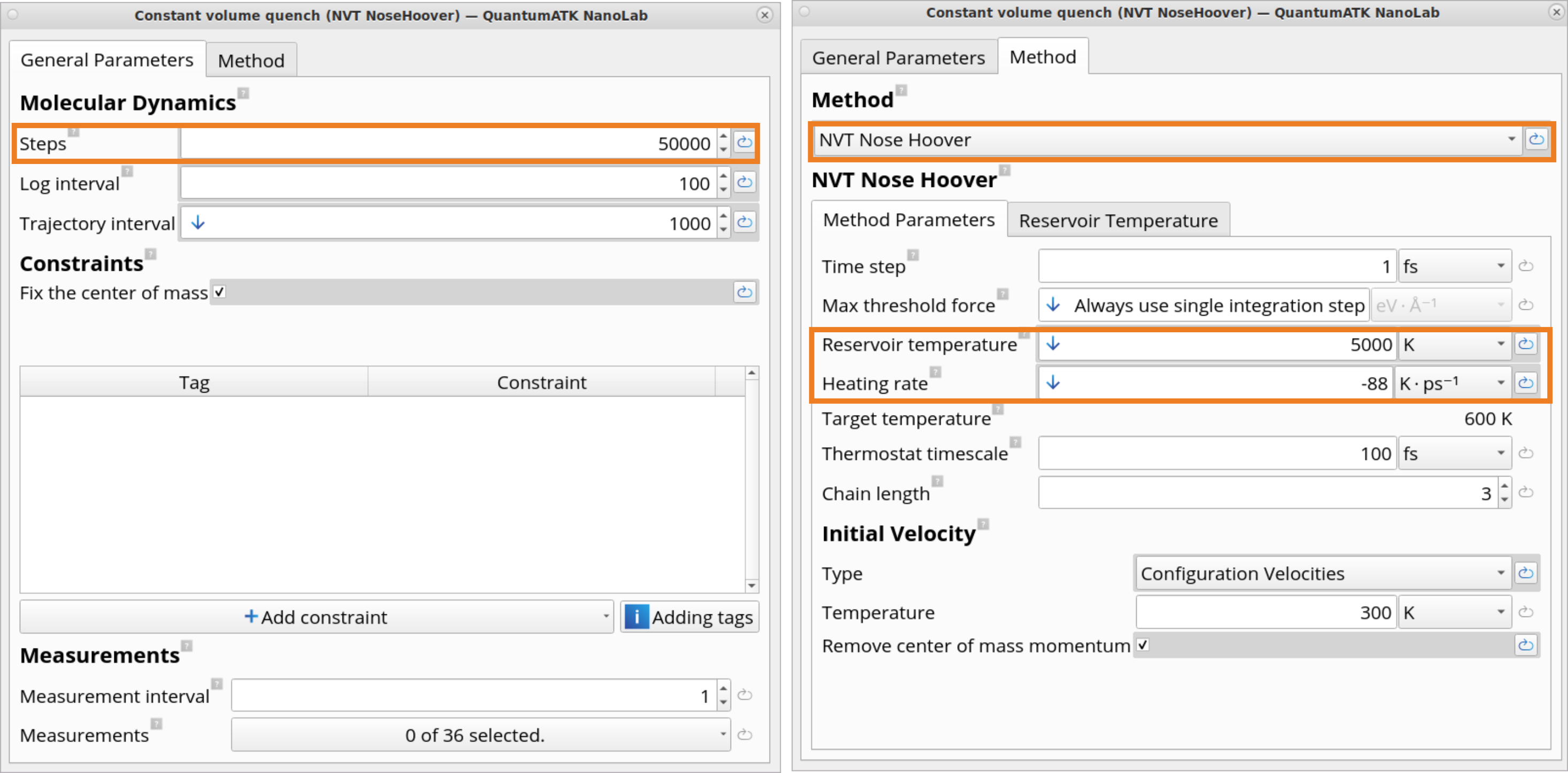
Click on the Constant volume quench (NVT NoseHoover) block, which contains settings for the NVT Nose Hoover type MD simulations to quench the structure from 5000 K to 600 K using -88\(Kps^{-1}\)Heating rate within 50 ps (50 000 MD steps with a time step of 1 fs). Use the settings set by the template.
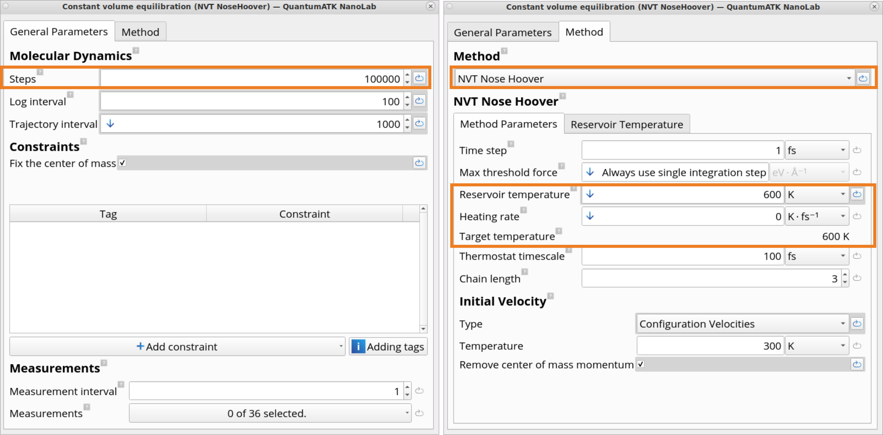
Click on the Constant volume equilibration (NVT NoseHoover) block, which defines settings for the NVT Nose Hoover type MD equilibration simulations. In this example, you will equilibrate the system for 100 ps at 600 K in order to reach a stable state where system’s temperature and energy are stable, thus allowing us to obtain meaningful RDF and ADF values.
Tip
In the Molecular Dynamics block, one can choose between various Molecular Dynamics methods: NVE Velocity Verlet, NVT Berendsen, NVT Bussi Donadio Parrinello, NVT Nose Hoover, Langevin, NPT Berendsen, NPT Bernetti Bussi, NPT Martyna Tobias Klein, Non Equilibrium Momentum Echange and Stress Strain. Read these technical notes on Molecular Dynamics to learn more.
In the Molecular Dynamics block, it is possible to edit a variety of MD parameters, such as a number of steps, time step, reservoir temperature, heating rate, target temperature, friction, velocity initialization type and temperature.
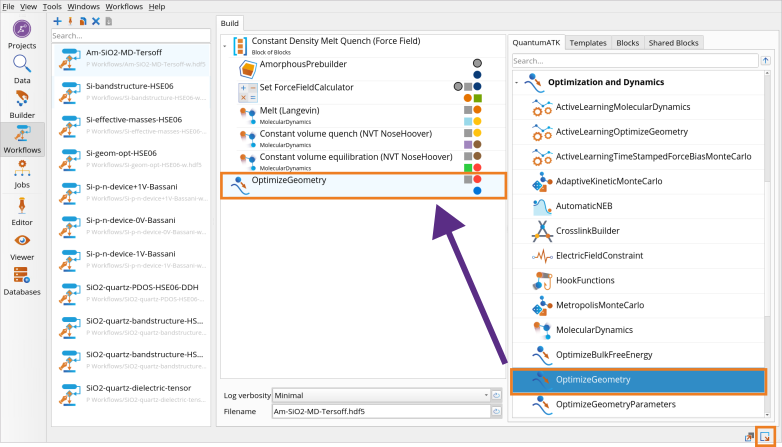
Go to the Block Catalog ‣ QuantumATK tab ‣ Optimization and Dynamics category on the right hand panel and drag-and-drop the OptimizeGeometry block to the middle Workflow Area ‣ Build tab.
Click on the OptimizeGeometry block to set the OptimizeGeometry to obtain the 0K structure of amorphous SiO2 using the same Tersoff_SiO_2007 Classical Force Field.
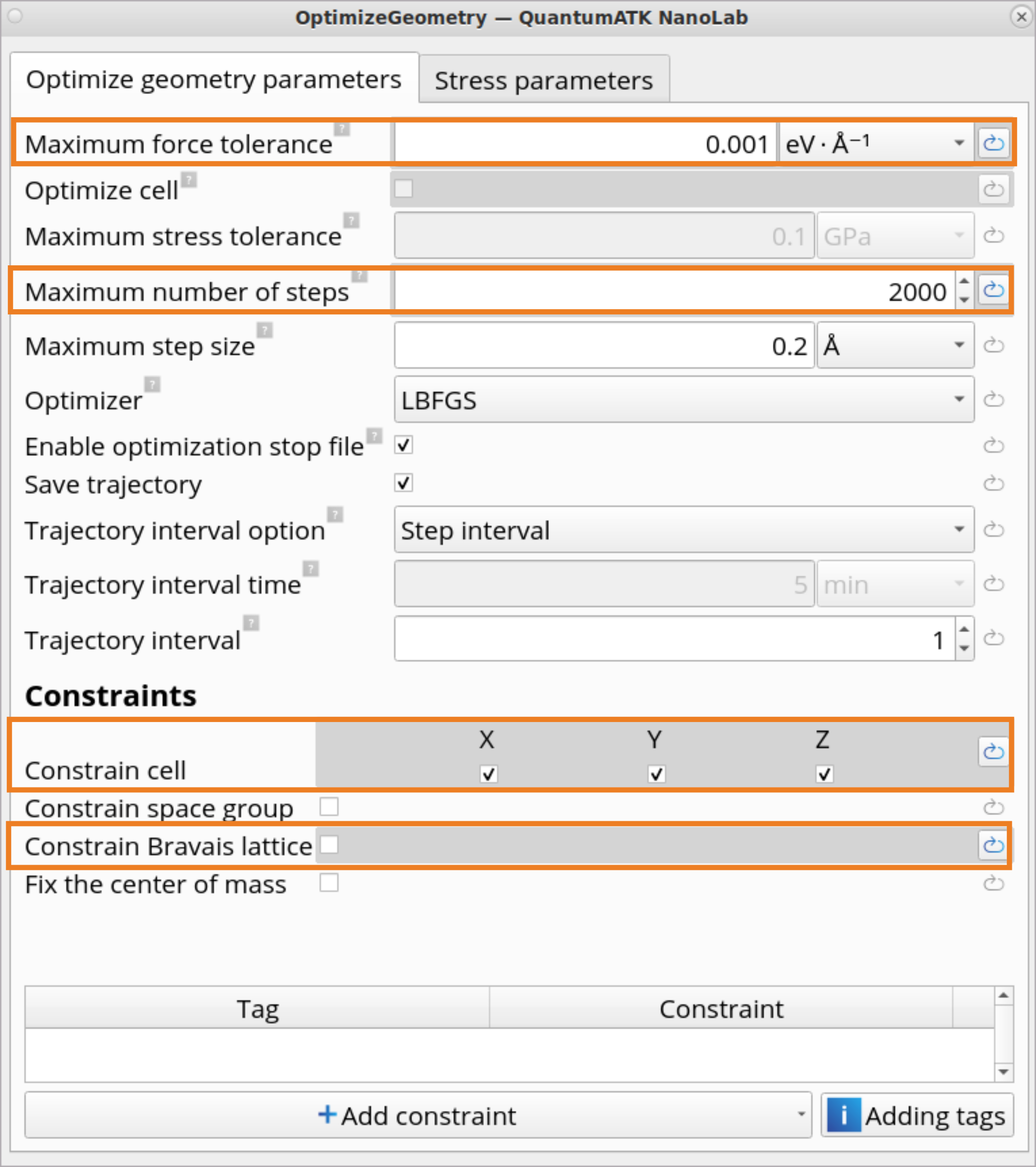
Set a tighter than default Force tolerance (0.001\(eV ⋅ Å^{-1}\)).
Increase Maximum number of steps to 2000, as many more optimization steps are needed when performing a geometry optimization with classical Force Fields.
Constrain cell in x, y and z directions and un-click Constrain Bravais lattice.
Note
Note, that when calculating electronic properties, it is important to perform a prior geometry optimization with DFT to get accurate electronic properties. In such a case, drag-and-drop the SetLCAOCalculator and additional OptimizeGeometry blocks to the workflow to set up the simulation.
Change the Workflow name in the Workflow Stash and Filename as needed (e.g., Am-SiO2-MD-Tersoff.hdf5).
Click on the Send content to other tools button and choose Jobs as a script to send the workflow to the Jobs tool in order to submit this job on a local machine or a remote cluster. It is recommended to use threading for Force Field simulations.
This also generates a Python script Am-SiO2-MD-Tersoff.py, based on this workflow. It can be opened and edited with the Editor tool and then sent to the Jobs tool.
Once the calculation has finished, we are ready to analyze the results.
Go to the Data View tool.
In the Data Sources, select the file Am-SiO2-MD-Tersoff.hdf5 and then in the Data View window double-click on the md object from the melt Langevin MD to open it with the Movie Tool.
Use the Movie Tool to investigate the temperature as well as the kinetic, potential and total energies, pressure, density and volume of the system as a function of simulation time, 30 ps in this case. You will observe the temperature oscillating around the set temperature (5000 K).
Simultaneously, an animation of the motion of the atoms is displayed. Right-click on the structure in the Movie tool to check the box Show bonds and use the Play button to see the evolution of structure throughout the MD simulation.
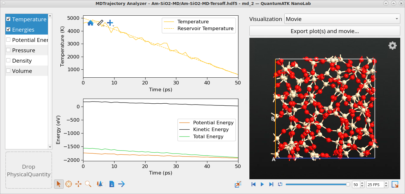
Come back to the Data View window and double-click on the md_2 object from the quench NVT Nose Hoover MD to open it with the Movie Tool.
Use the Movie Tool to investigate the temperature as well as the kinetic, potential and total energies, pressure, density and volume of the system as a function of simulation time, 50 ps in this case. The temperature is gradually reduced from 5000 K to ~ 600 K as set in the workflow.
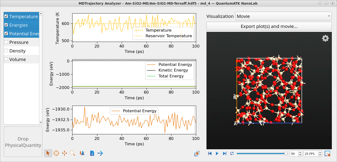
Come back to the Data View window and double-click on the md_4 object from the NVT Nose Hoover type MD equilibration simulations to open it with the Movie Tool. The temperature fluctuates around the set value of 600 K, and the energies also fluctuate around their equilibrium values, indicating that the system is stable. This allows us to obtain meaningful RDF and ADF values from this trajectory.
Come back to the Data View window and right-click on the md_4 object from the NVT Nose Hoover type MD equilibration simulations to open it with the Molecular Dynamics Analyzer to plot calculated RDF and ADF for amorphous SiO2.
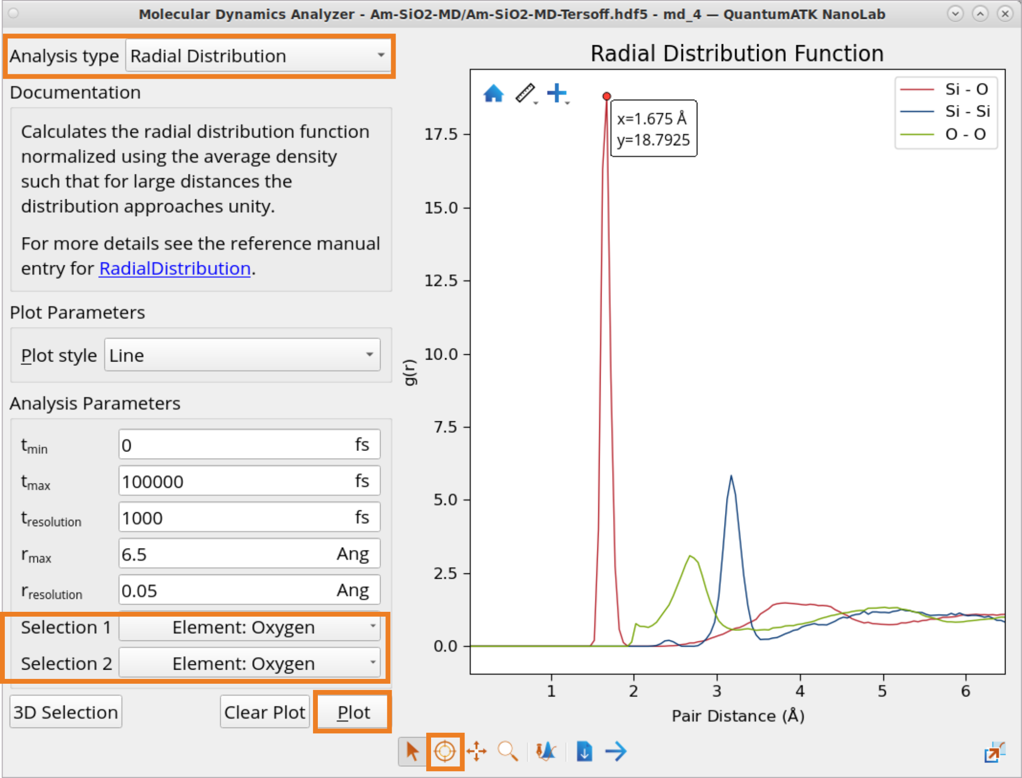
In order to plot RDF:
Click on Analysis type selection box and choose to plot Radial Distribution.
Click on Selection 1 and Selection 2 boxes to choose for which element combinations to plot RDF.
Click Plot to generate RDF plots for Si-O, Si-Si and O-O one-by-one.
Click on the Inspect tool to examine the exact RDF values.
Note
Calculated radius values for the 1st coordination sphere obtained from the RDF plot: \(r_{Si-O}\) = 1.675 Å, \(r_{Si-Si}\) = 3.175 Å and \(r_{O-O}\) = 2.675 Å are in a reasonably good agreement with experimental values for fused silica at 300 K: \(r_{{Si-O}_{exp}}\) = 1.62 Å, \(r_{{Si-Si}_{exp}}\) = 3.12 Å and \(r_{{O-O}_{exp}}\) = 2.65 Å [1].
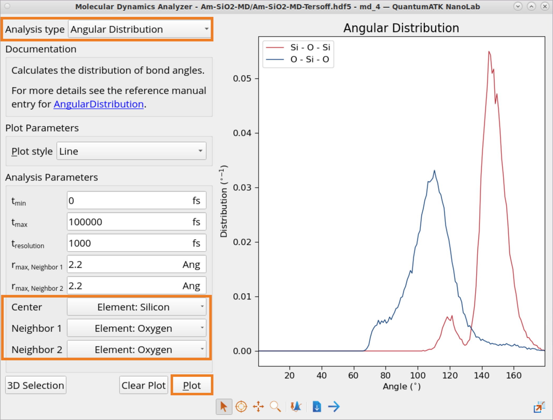
In order to plot ADF:
Click on Analysis type selection box and choose to plot Angular Distribution.
Click on Center, Neighbor 1 and Neighbor 2 boxes to choose for which element combinations to plot ADF.
Click Plot to generate ADF plots for Si-O-Si and O-Si-O one-by-one.
Note
Calculated angle values for all the coordination spheres obtained from the ADF plot: \(\theta_{O-Si-O}\) = 110.5° and \(\theta_{Si-O-Si}\) = 144.5° are also in a reasonably good agreement with experimental values for fused silica at 300 K: \(\theta_{{O-Si-O}_{exp}}\) = 109.7° and \(\theta_{{Si-O-Si}_{exp}}\) = 152.0° [2].
Come back to the Data View window and right-click on the optimize_trajectory object from the final geometry optimization at 0 K and to see the evolution of structure throughout the geometry optimization simulation. The geometry converged in 611 steps.
Right-click on the the optimized geometry optgeom in Data View and choose to Open with Builder. The optimized geometry will be automatically saved in the BuilderStash, so you could use it for other simulations.

 Workflow Builder, follow the step-by-step protocol described below. Here, we will use a classical Force Field Tersoff_SiO_2007.
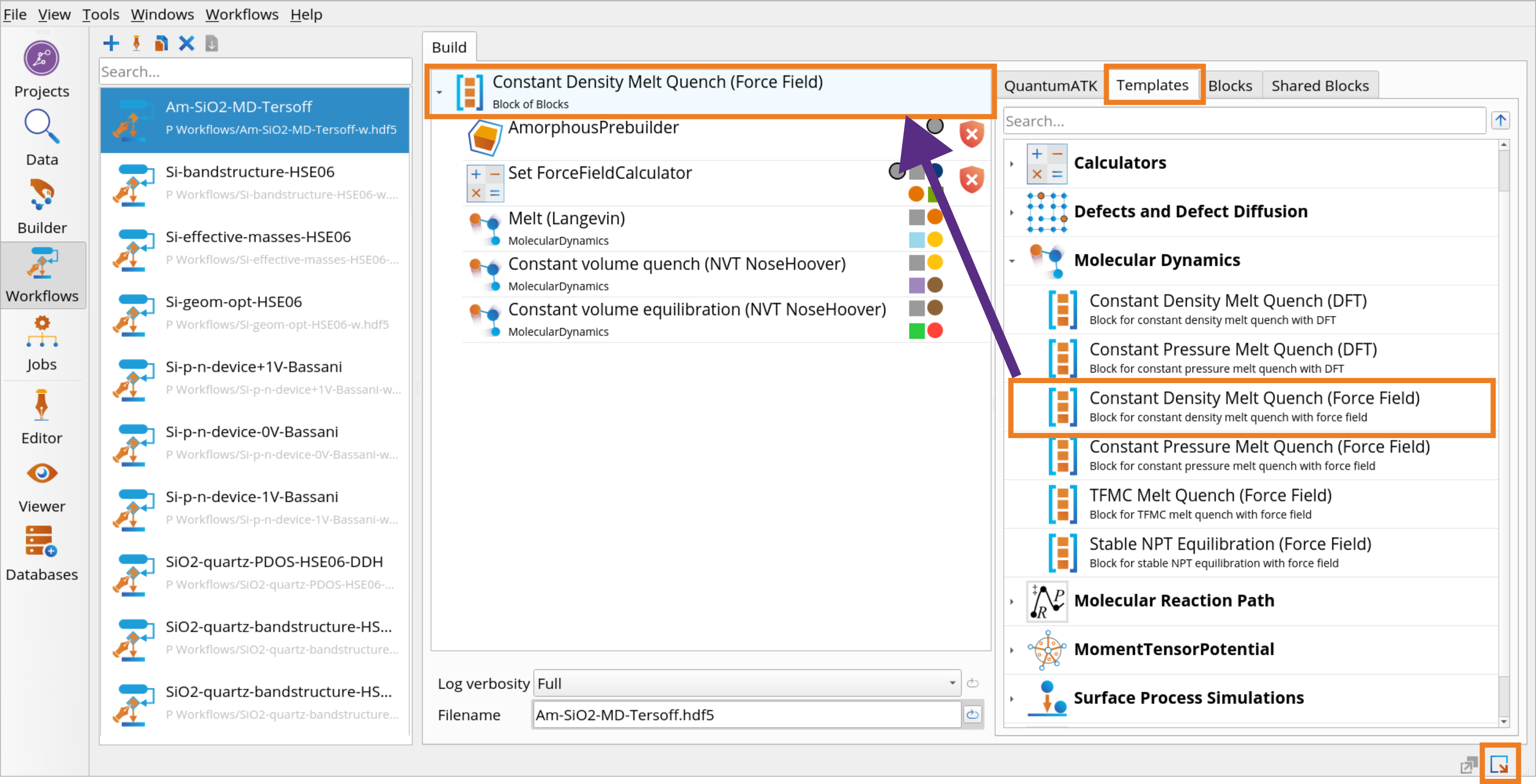
 SetLCAOCalculator and additional OptimizeGeometry blocks to the workflow to set up the simulation.
 Send content to other tools button and choose Jobs as a script to send the workflow to the
  Jobs tool in order to submit this job on a local machine or a remote cluster. It is recommended to use threading for Force Field simulations.
 Editor tool and then sent to the
  Data View tool.
 md object from the melt Langevin MD to open it with the Movie Tool.
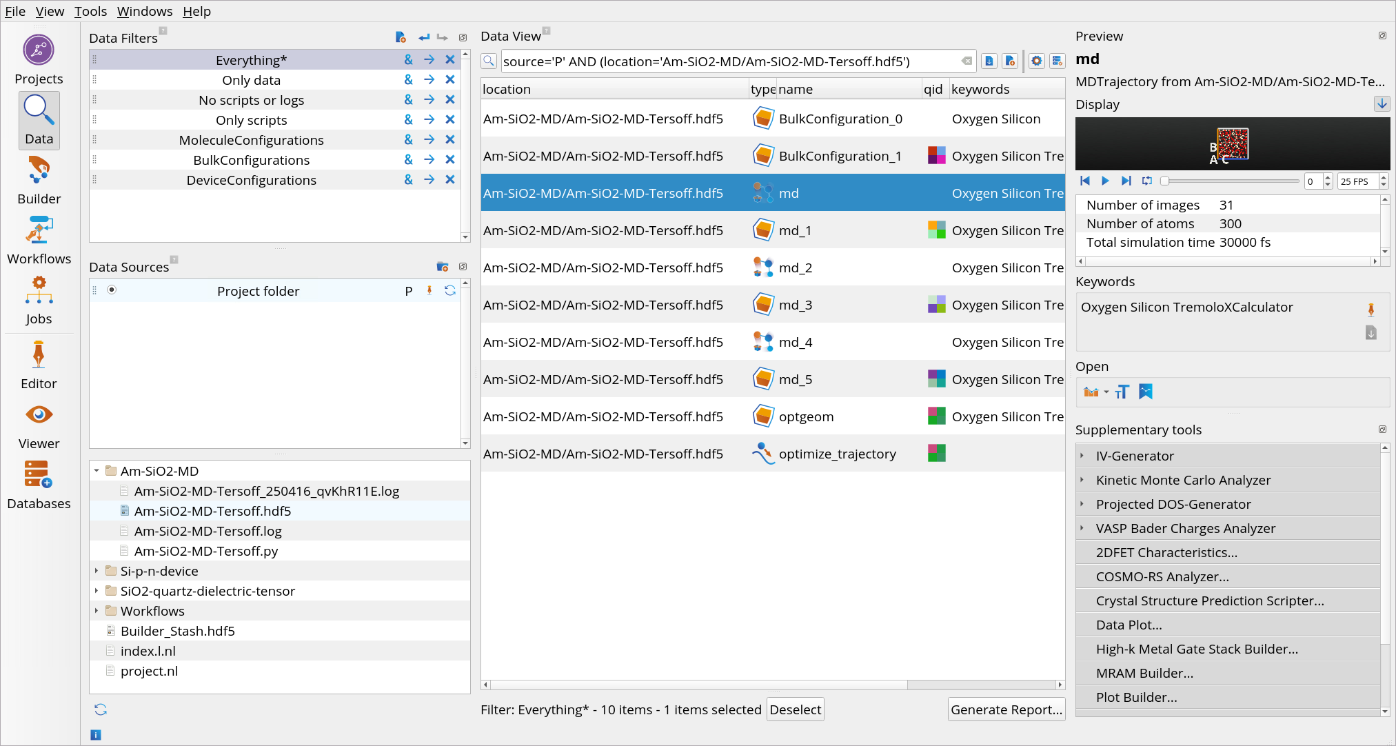
 Play button to see the evolution of structure throughout the MD simulation.
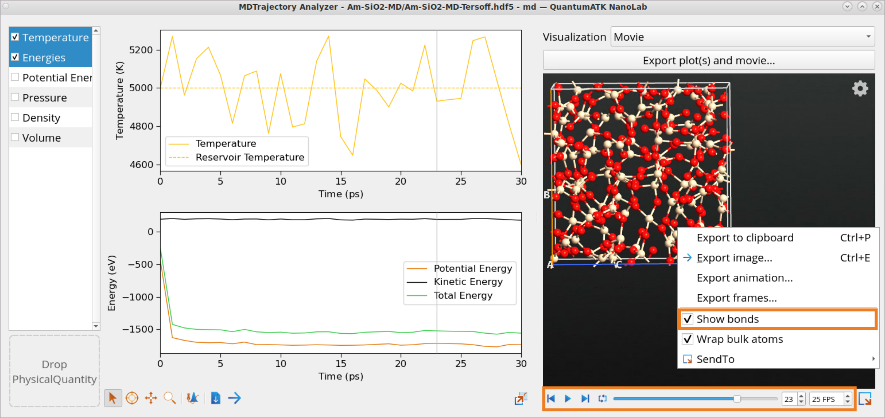
Inspect tool to examine the exact RDF values.
 optimize_trajectory object from the final geometry optimization at 0 K and to see the evolution of structure throughout the geometry optimization simulation. The geometry converged in 611 steps.
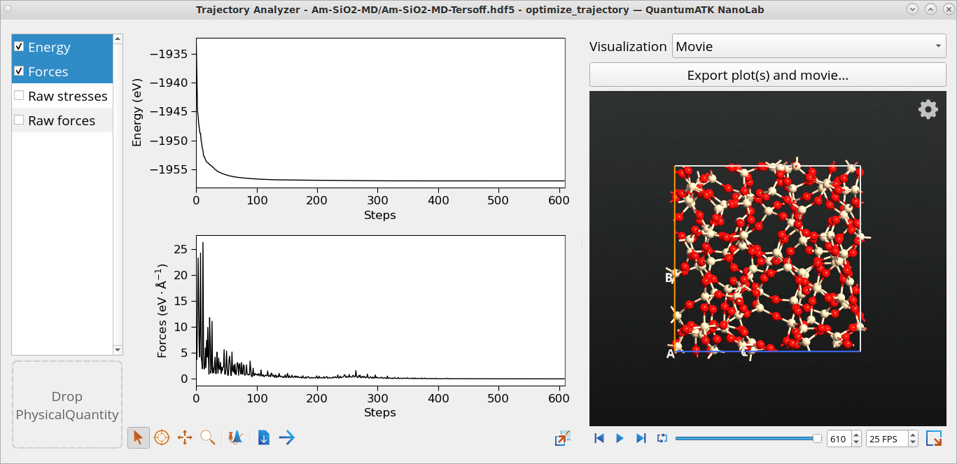
 optgeom in Data View and choose to Open with Builder. The optimized geometry will be automatically saved in the
  Builder Stash, so you could use it for other simulations.