Elastic constants
QuantumATK provide a very simple way to set up and execute calculations of the elastic constants for arbitrary bulk configurations. The method is generalized and can easily be used with density functional theory (ATK-DFT), semi-empirical methods (ATK-SE), or classical potentials (ATK-ForceField). In this tutorial, you will learn how to calculate elastic constants with QuantumATK.
Note
In a bulk solid, the elastic constants relate the linear response of the stress tensor \(\boldsymbol{\sigma}\) to an external strain \(\boldsymbol{\varepsilon}\) on the system. The elastic constants thereby describe the directional stiffness of the material under specific types of deformations. More general moduli, such as bulk, shear, or Young’s modulus, can also be calculated.
All of these quantities characterize the mechanical properties of a solid. In addition, elastic constants and moduli are often employed as fitting observables for parameterization of classical potentials.
Methodology
The stress and strain tensors are always symmetric 3x3 matrices, and they can therefore be expressed more compactly as 6-vectors, using the so-called Voigt notation:
and
The linear response of the stress vector to a given strain vector can then be written as
where the symmetric 6x6 matrix \(\boldsymbol{C}\) contains the elastic constants.
Depending on the crystal symmetry, the number of independent entries in \(\boldsymbol{C}\) can be reduced further. For instance, in a cubic crystal only three entries, \(C_{11}\), \(C_{12}\), and \(C_{44}\), are independent:
To obtain the elastic constants, one should apply small deformations, \(\eta\), to the simulation cell along selected strain vectors, and calculate the resulting stress vectors. The linear stress contribution is obtained by fitting the \(\sigma_i(\eta)\) curves of each Voigt stress component and for every strain vector. The independent elastic constants are then calculated as the least-squares solution to a linear system of equations, taking the crystal symmetry into account.
Note
For the calculation of elastic constants, QuantumATK employs the Lagrangian strain and stress tensors instead of the corresponding physical tensors.
To minimize the number of stress calculations, QuantumATK uses the Universal Linearly-Independent Coupling Strain (ULICS) vectors (Ref. [1]). For each strain vector, typically three deformations (\(-\eta\), 0, \(+\eta\)), centered at the reference configuration (\(\eta=0\)), are applied.
Important
For configurations with more than one atom in the cell, the atomic positions of each strained cell must be optimized before the stress is calculated; QuantumATK automatically takes care of this. You should however ensure that the cell vectors (and atomic positions) of the reference configuration are well optimized before starting the calculation of the elastic constants.
Calculating elastic constants using classical potentials
You will now perform an elastic constant calculation based on classical potentials, using ATK-ForceField. The advantage of of classical potentials, apart from the calculation speed, is that that most properties, such as energies, forces and stress, are smooth functions of the coordinates. This makes calculation of elastic constants particularly robust with respect to the setting sused for calculating the strain.
Two examples will be considered:
A bulk silicon crystal, using the Stillinger–Weber potential [2].
SiO2 \(\alpha\)-quartz, using the “Pedone2006 Fe2” potential [3].
Bulk silicon
Open the QuantumATK Builder  and use
to add “Silicon (alpha)” to the Stash. Then send the configuration to the
Script Generator
and use
to add “Silicon (alpha)” to the Stash. Then send the configuration to the
Script Generator  and do the following:
Add a New Calculator
 block.
Select ATK-ForceField and the “Stillinger_Weber_Si_1985” potential.
Note
For QuantumATK-versions older than 2017, the ATK-ForceField calculator can be found under the name ATK-Classical.
Add a
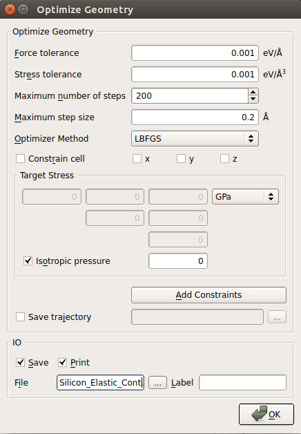
 object to the script and edit it:
select sufficiently accurate settings for maximum force and maximum stress, e.g. 0.001 eV/Å for the force and 0.001 eV/Åsup:3 for the stress;
uncheck the “Constrain cell” check box to enable optimization of the cell vectors;
select LBFGS as the optimizer method.
Back in the Scripter, add an
 block
Open the block to set up the analysis.
block
Open the block to set up the analysis.
The first set of parameters and options refer to the stress/strain calculation:
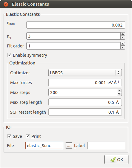
- Parameter: \(\eta_{max}\)
Specifies the maximum deformation magnitude applied to the cell. A sufficiently large value should be chosen to achieve a significant variation in stress, but small enough to remain essentially within the linear regime. The default value of 0.002 is in most cases a good choice. Elastic constants calculated with classical potentials are in general not too sensitive to this parameter.
- Parameter: \(n_\eta\)
Specifies the number of intermediate deformations between \(-\eta_{max}\) and \(+\eta_{max}\) for every strain vector. A higher value, together with a higher-order fit (as specified by the next parameter), may help to filter out possible non-linear contributions, but also increases the number of calculations that need to be performed. The default value is 3 and usually works well.
- Parameter: Fit order
Specifies the highest polynomial order in the stress vs. \(\eta\) fitting procedure, which should be smaller than \(n_\eta\). For evaluation of the elastic constants, only the linear contribution is used.
- Option: Enable symmetry
Allows QuantumATK to detect the crystal symmetry and calculate only the independent constants for this lattice symmetry. Otherwise, all 21 constants of the upper triangle of the \(\boldsymbol{C}\) matrix are treated as independent.
The remaining settings are related to the force optimization (of the atomic coordinates) that can be invoked before the stress of each strained system is calculated:
- Option: Optimizer
Sets the optimizer method. If you select “None”, no force optimization is carried out before the stress is calculated, which is the fastest, but least accurate option. If there is only one atom in the unit cell, there is no need for an optimization of the internal coordinates and the optimizer is automatically disabled.
- Parameters for force and stress minimization
The remaining parameters control the optimizer setttings. These options are in fact the same as in the OptimizeGeometry
object. While most of these
parameters are only relevant in special cases, the “Max forces” parameter should be
chosen sufficiently accurate. The default value of 0.005 eV/Å (which is 10x lower
than the usual default in QuantumATK) represents a good balance between accuracy and efficiency.
Since the example at hand uses fast ATK-ForceField calculations, you can easily afford
to reduce this value even further to 0.001 eV/Å to achieve a higher precision.
Execute the calculation by sending the script to the Job Manager  ,
again using the
,
again using the  button. You may be asked to save the script again.
Click the
button. You may be asked to save the script again.
Click the  button to start the job. It takes around five seconds to finish on a laptop.
Analysis of the results
You can find information about the calculation and results in the log file*. As you see, QuantumATK has correctly recognized the cubic symmetry of the FCC silicon crystal and calculates only the three independent elastic constants:
+------------------------------------------------------------------------------+
| Calculating elastic constants for the given bulk configuration               |
+------------------------------------------------------------------------------+
| Detected space group number:    227                                          |
| Detected lattice symmetry:      Cubic                                        |
| This lattice symmetry has 3 independent elastic constants:                   |
| C11  C12  C44                                                                |
+------------------------------------------------------------------------------+
The elastic constants matrix is printed at the bottom of the log file, and is in excellent agreement with literature results using the Stillinger–Weber potential [4]:
Tip
The log file also records more detailed analysis of the elastic constant matrix. It contains the elastic compliance matrix, which is the inverse of the elastic constants matrix. More general moduli, such as bulk, shear or Young’s modulus, are also calculated from the elastic constants. Be aware tha there are three different definitions of bulk and shear modulus, according to the slightly different formulae from Voigt and Reuss. All of them are listed in the log output for comparison.
SiO2 quartz
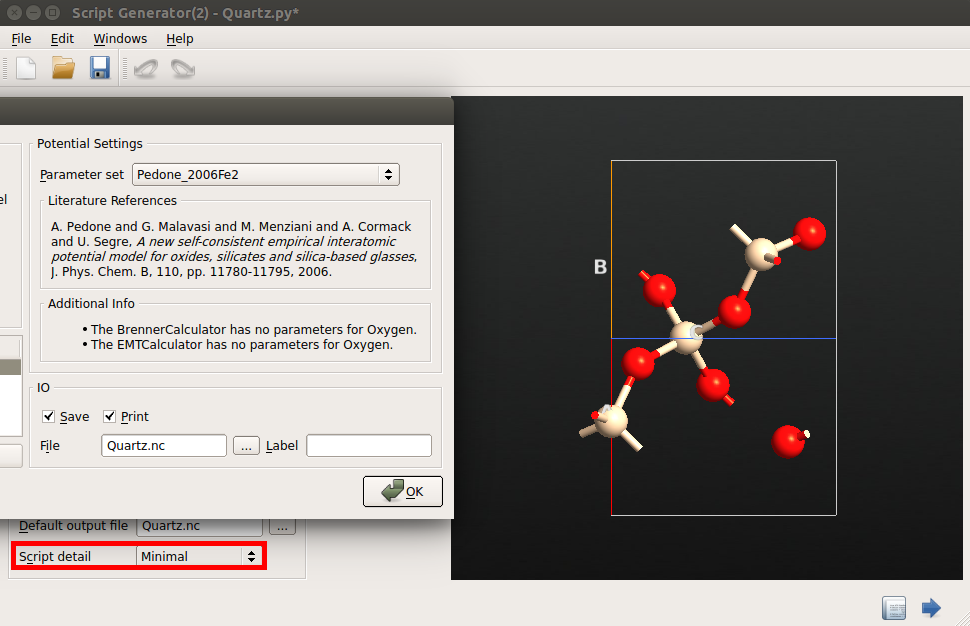
You can use the same method to compute the elastic properties of more complex crystals, such as SiO2 \(\alpha\)-quartz. Follow the same steps above and select the “Pedone2006_Fe2” potential , which is from Ref. [3].
Accurate long-range electrostatics
After setting up the script in the Script Generator, change the Script Detail
setting in the Global IO field from “Minimal” to “Show defaults”, and
transfer the script to the Editor  in order to make one small modification.
In the calculator block, you will find that all the pair potentials are now
individually listed and added to the potential set (this is a result of the
“Show defaults” setting).
in order to make one small modification.
In the calculator block, you will find that all the pair potentials are now
individually listed and added to the potential set (this is a result of the
“Show defaults” setting).
The Pedone potential includes long-range electrostatic interations. You can manually
increase the cutoff distance for these interactions (r_cut). To achieve a high
accuracy of the stress calculation, you should change this parameter from the default
of 9.0 Å to a larger value of 15 Å, to account for the long-range nature of the
Coulomb potential:
potentialSet.setCoulombSolver(CoulombDSF(r_cut=15.0*Angstrom, alpha = 0.2))
calculator = TremoloXCalculator(parameters=potentialSet)
calculator.setInternalOrdering("default")
This will affect the speed of the calculations, but since the elastic constants calculation does not involve extensively long simulations, you will hardly notice it.
Results
Performing the calculation will give the following results:
+------------------------------------------------------------------------------+
| Elastic Constants in GPa                                                     |
+------------------------------------------------------------------------------+
|    86.55       8.71      11.16     -18.36       0.00       0.00              |
|               86.55      11.16      18.36       0.00       0.00              |
|                         106.67       0.00       0.00       0.00              |
|                                     49.41       0.00       0.00              |
|                                                49.41     -18.36              |
|                                                           38.92              |
+------------------------------------------------------------------------------+
Due to the rhombohedral symmetry, there are six independent constants, \(C_{11}, C_{12}, C_{13}, C_{14}, C_{33}\) and \(C_{44}\). All values reproduce very well the results of the original publication, Ref. [3].
Calculate elastic constants using DFT
Finally, you will perform a calculation of the elastic constants of silicon using density functional theory. The framework outlined above can be used again – you just need to replace the calculator such that is uses ATK-DFT with GGA exchange correlation.
Use again the Builder to create the silicon structure and send it to the
Script Generator. Add the New Calculator , OptimizeGeometry
and ElasticConstants blocks.
To obtain numerically precise stress differences between the strained conformations, we generally have to employ some slightly tighter calculator settings than the defaults:
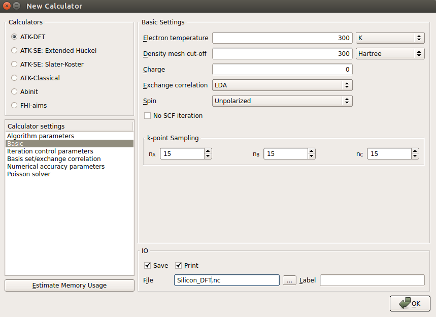
Choose ATK-DFT as the calculator, and set the following parameters in Basic:
set the grid mesh cut-off to 300 Hartree;
set k-point sampling to 15x15x15.
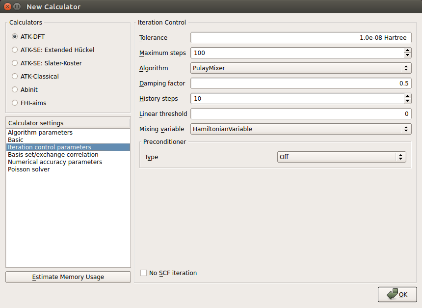
In the Iteration control parameters tab:
set the tolerance parameter to 1.0e-08;
set the damping factor to 0.5 and the number of history steps to 10.
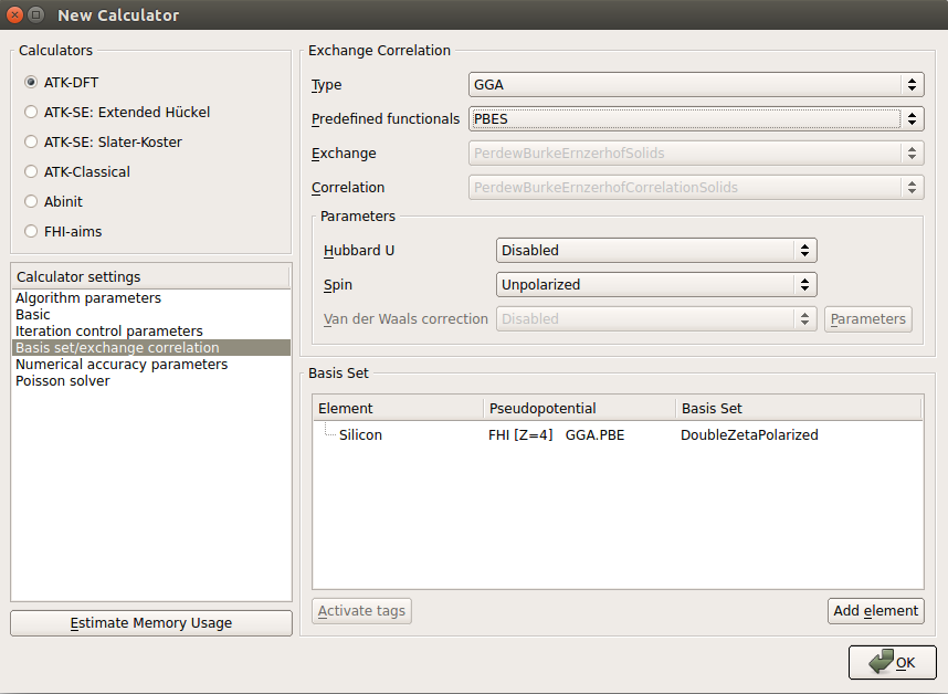
In the Basis set/exchange correlation tab use the PBEsol functional, which offers very reliable DFT predictions of bulk moduli and related quantities:
choose GGA for the exchange-correlation type;
select in PBES in the list of predefined functionals;
The settings in the OptimizeGeometry and ElasticConstants blocks should be almost identical to the ones chosen for the classical potentials, except that the \(\eta_{max}\) value in the ElasticConstants settings should be 0.003 (which means that a larger strain will be employed, resulting in a more pronounced change in the stress).
This calculation takes only about 10 minutes to finish. The calculated elastic constants are
+------------------------------------------------------------------------------+
| Elastic Constants in GPa                                                     |
+------------------------------------------------------------------------------+
|   161.02      65.22      65.22       0.00       0.00       0.00              |
|              161.02      65.22       0.00       0.00       0.00              |
|                         161.02       0.00       0.00       0.00              |
|                                     75.68       0.00       0.00              |
|                                                75.68       0.00              |
|                                                           75.68              |
+------------------------------------------------------------------------------+
The results are in reasonably good agreement with the experimental values, Ref. [5], which are listed below:
References