Bandstructure¶

class Bandstructure(configuration, route=None, points_per_segment=None, kpoints=None, bands_above_fermi_level=None, projection_list=None, processes_per_kpoint=None, method=None, interpolation_method=None, diagonalization_method=None)¶

Analysis class for calculating the bandstructure for a bulk configuration.

Parameters:

configuration (BulkConfiguration) – The bulk configuration with an attached calculator for which to calculate the bandstructure.
route (list of str) – The route to take through the Brillouin-zone as a list of symmetry points of the unit cell, e.g. ['G', 'X', 'G']. This option is mutually exclusive to kpoints.
Default: Unit-cell dependent route.
points_per_segment (Positive int) – The number of points per segment of the route. This option is mutually exclusive to kpoints.
Default: 20.
kpoints (list of lists of floats) – A list of 3-dimensional fractional k-points at which to calculate the energies of the bands e.g. [[0.0, 0.0, 0.0], [0.0, 0.0, 0.1], ...]. The shape is (K, 3) where K is the number of k-points. This option is mutually exclusive to route, and points_per_segment.
Default: Unit-cell dependent route.
bands_above_fermi_level –
Deprecated: from v2023.09, see diagonalization_method and FullDiagonalizationSolver instead.
projection_list (ProjectionList) – A projection list object defining a projection.
Default: If no projection list is specified all orbitals will be used.
processes_per_kpoint (int | None) – The number of processes to use per kpoint.
Default: For PlaneWaveCalculator, the default is the same number of processes per k-point as used in the SCF calculation. Otherwise, the default is 1.
method –
Deprecated: from v2023.09, use interpolation_method parameter instead.
interpolation_method (None | Full | KDotPExpansion1D | KDotPExpansion3D) –
The method used for the bandstructure calculation.

Default is to perform an exact eigenvalue solution for each k-point.

Alternatively, the k.p expansion method can be use to interpolate the eigenvalues at the requested k-points using the exact eigensolution computed for a small subset of the k-points. There are two modes for the k.p method. 1) Using KDotPExpansion1D, for each bandstructure path segment, a few exact eigensolution are calculated and the eigenvalues of the remaining k-points are interpolated using a 1D correction term. 2) Using KDotPExpansion3D, the eigenvalues for the requested k-points are interpolated from exact solution on a 3D grid. The bands, grid and wave functions of a previous ground state computation can be used in this approach.

Default: Full meaning that all k-points will be calculated exactly.
diagonalization_method –
Method used for diagonalizing the hamiltonian.

This parameter allows to choose between a full diagonalization solver and an iterative subspace solver. The full diagonalization solver evaluates all bands from the lowest energy one to a given number of bands above fermi level. The iterative subspace solver allows to evaluate a given number of bands around fermi level, or around an energy of choice.

The full diagonalization solver is more robust, but can be proibitively expensive for very large systems.

The iterative solver can deal with very large systems (tens of thousands atoms and beyond) and greatly outperforms when calculating a small number of eigenvalues, but it is also inherently less robust.

Note: the exact method used when selecting FullDiagonalizationSolver is defined by the calculator (see AlgorithmParameters). IterativeDiagonalizationSolver is not supported for PlaneWaveCalculator

Default: FullDiagonalizationSolver

Type:

FullDiagonalizationSolver | IterativeDiagonalizationSolver

conductionBandEdge()¶

Calculate the conduction band edge.

Returns:: The conduction band edge.
Return type:: PhysicalQuantity of type energy

directBandGap()¶

Calculate the direct band gap.

Returns:: The direct band gap.
Return type:: PhysicalQuantity of type energy

energyZero()¶

The energy zero is equal to the Fermi level. For fixed spin moment calculations it is the average of the Fermi level for spin up and spin down.

Returns:: The energy zero.
Return type:: PhysicalQuantity of type energy

evaluate(spin=None)¶

Return the bandstructure for a given spin.

Parameters:: spin (Spin.Up | Spin.Down | Spin.All) – The spin the bandstructure should be returned for. Must be either Spin.Up or Spin.Down, or for noncollinear calculations Spin.All.
Default: Spin.All
Returns:: The eigenvalues for the specified spin. The shape is (K, B) or (S, K, B) where S is the number of spins, K is the number of k-points, and B is the number of bands.
Return type:: PhysicalQuantity of type energy | list of PhysicalQuantity of type energy

fermiLevel(spin=None)¶

Parameters:: spin (Spin.Up | Spin.Down | Spin.All) – The spin the Fermi level should be returned for. Must be either Spin.Up, Spin.Down, or Spin.All. Only when the band structure is calculated with a fixed spin moment will the Fermi level depend on spin.
Default: Spin.All
Returns:: The Fermi level in absolute energy.
Return type:: PhysicalQuantity of type energy

fermiTemperature()¶

Returns:: The Fermi temperature used in this bandstructure.
Return type:: PhysicalQuantity of type temperature

indirectBandGap()¶

Calculate the indirect band gap.

Returns:: The indirect band gap.
Return type:: PhysicalQuantity of type energy

interpolationMethod()¶

Returns:: The method used for the bandstructure calculation.
Return type:: None | Full | KDotPExpansion1D | KDotPExpansion3D

kpoints()¶

Returns:: The list of 3-dimensional fractional k-points at which the energies of the bands are calculated. The shape is (K, 3) where K is the number of k-points.
Return type:: list of lists of floats

metatext()¶

Returns:: The metatext of the object or None if no metatext is present.
Return type:: str | None

method()¶

Returns:: The method used for the bandstructure calculation.
Return type:: None | Full | KDotPExpansion1D | KDotPExpansion3D

Deprecated: Use interpolationMethod() instead.

nlinfo()¶

Returns:: Structured information about the Bandstructure.
Return type:: dict

nlprint(stream=None)¶

Print a string containing an ASCII table useful for plotting the AnalysisSpin object.

Parameters:: stream (python stream) – The stream the table should be written to.
Default: NLPrintLogger()

processesPerKPoint()¶

Deprecated: from v2019

Returns:: The number of processes per k-point used in the calculation.
Return type:: int > 0

route()¶

Returns:: The route through the Brillouin-zone as a list of symmetry points of the unit cell.
Return type:: list of str

setMetatext(metatext)¶

Set a given metatext string on the object.

Parameters:: metatext (str | None) – The metatext string that should be set. A value of “None” can be given to remove the current metatext.

uniqueString()¶: Return a unique string representing the state of the object.

valenceBandEdge()¶

Calculate the valence band edge.

Returns:: The valence band edge.
Return type:: PhysicalQuantity of type energy

Usage Examples¶

Calculate the bandstructure of silicon and save it to a file:

# -------------------------------------------------------------
# Bulk Configuration
# -------------------------------------------------------------
lattice = FaceCenteredCubic(5.4306*Angstrom)
elements = [Silicon, Silicon]
fractional_coordinates = [[ 0.  ,  0.  ,  0.  ],
                          [ 0.25,  0.25,  0.25]]
bulk_configuration = BulkConfiguration(
    bravais_lattice=lattice,
    elements=elements,
    fractional_coordinates=fractional_coordinates
    )

# -------------------------------------------------------------
# Calculator
# -------------------------------------------------------------
basis_set = [CerdaHuckelParameters.Silicon_GW_diamond_Basis]
hamiltonian_parametrization = HuckelHamiltonianParametrization(
    basis_set=basis_set)
k_point_sampling = MonkhorstPackGrid(9,9,9)
numerical_accuracy_parameters = NumericalAccuracyParameters(
    k_point_sampling=k_point_sampling,
    density_mesh_cutoff=10.0*Hartree,
    )
calculator = SemiEmpiricalCalculator(
    hamiltonian_parametrization=hamiltonian_parametrization,
    numerical_accuracy_parameters=numerical_accuracy_parameters,
    )
bulk_configuration.setCalculator(calculator)
bulk_configuration.update()

# -------------------------------------------------------------
# Bandstructure
# -------------------------------------------------------------
bandstructure = Bandstructure(
    configuration=bulk_configuration,
    route=['G', 'X'],
    points_per_segment=40,
    bands_above_fermi_level=4
    )

# Read the valence and conduction band edges wrt. the Fermi level
edge_valence = bandstructure.valenceBandEdge()
edge_conduction = bandstructure.conductionBandEdge()
print(edge_valence)
# Read the direct and indirect band gaps
gap_direct   = bandstructure.directBandGap()
gap_indirect = bandstructure.indirectBandGap()
print(gap_indirect)
# Print out results
print('Valence band maximum    = %.2f eV' % edge_valence.inUnitsOf(eV))
print('Conduction band minimum = %.2f eV' % edge_conduction.inUnitsOf(eV))
print('Direct band gap   = %.2f eV' % gap_direct.inUnitsOf(eV))
print('Indirect band gap = %.2f eV' % gap_indirect.inUnitsOf(eV))

si_band.py

Notes¶

To export the data of a Bandstructure, use the method nlprint.

Note that the k-points are given in units of the reciprocal vectors \({\bf k}_A\) , \({\bf k}_B\) , and \({\bf k}_C\). E.g. the symmetry point \(X\) have the fractional k-point coordinates \((\frac{1}{2}, 0, \frac{1}{2})\) since it is described by \(X = \frac{1}{2}{\bf k}_A + \frac{1}{2}{\bf k}_C\) .

A query method for the symmetry points of the Brillouin zone can be found in Common methods of the Bravais Lattices class.

For bands_above_fermi_level set to a valid integer \(N_{\text{ba}}\), the total number of bands above the Fermi level will be \(N_{\text{ba}}\) for the spin type unpolarized and \(2 N_{\text{ba}}\) for polarized and noncollinear. This is because there is one spin channel in the former case and two spin channels in the latter two cases. Spin-orbit calculations are categorized as non-collinear calculations and therefore follow the same band selection as noncollinear. The case where bands_above_fermi_level is 1 is illustrated in Fig. 144. Note, that all bands below the Fermi level are always selected.

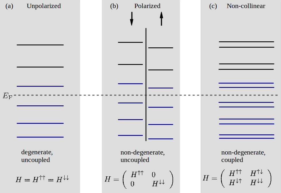
../../../_images/spin_type_bands_above.png — Fig. 144 The total number of bands selected (blue lines) by specifying 1 band above the Fermi level for **(a)** an unpolarized, **(b)** a polarized, and **(c)** a non-collinear calculation. The Fermi level \(E_{\text{F}}\) is shown as a horizontal dashed gray line. The vertical separation line in **(b)** signifies that the bands can be categorized according to spin up or down since there is no coupling. The structure of the Hamiltonian for each of the 3 spin types is shown at the bottom.¶