DynamicalMatrix

class DynamicalMatrix(configuration, filename, object_id, calculator=None, repetitions=None, atomic_displacement=None, acoustic_sum_rule=None, finite_difference_method=None, constraints=None, constrain_electrodes=None, use_equivalent_bulk=None, max_interaction_range=None, force_tolerance=None, processes_per_displacement=None, log_filename_prefix=None, use_wigner_seitz_scheme=None, use_symmetry=None, polar_phonon_splitting_parameters=None, use_internal_coordinates=None, bond_list=None, symmetrize=None)

Constructor for the DynamicalMatrix object.

Parameters:

• configuration (BulkConfiguration | MoleculeConfiguration | DeviceConfiguration) – The configuration for which to calculate the dynamical matrix.

• calculator (Calculators) – The calculator to be used in the dynamical matrix calculations.
  Default: The calculator attached to the configuration.

• filename (str) – The full or relative path to save the results to. See nlsave().

• object_id (str) – The object id to use when saving. See nlsave().

• repetitions (Automatic | list of ints) – The number of repetitions of the system in the A, B, and C-directions given as a list of three positive integers, e.g. [3, 3, 3], or Automatic. Each repetition value must be odd.
  Default: Automatic

• atomic_displacement (PhysicalQuantity of type length) – The distance the atoms are displaced in the finite difference method.
  Default: 0.01 * Angstrom

• acoustic_sum_rule (bool) – Control if the acoustic sum rule should be invoked.
  Default: True

• finite_difference_method (Forward | Central) – The finite difference scheme to use.
  Default: Central

• constraints (list of type int) – List of atomic indices that will be constrained, e.g. [0, 2, 10].
  Default: None

• constrain_electrodes (bool) – Control if the electrodes and electrode extensions should be constrained in case of a DeviceConfiguration.
  Default: False

• use_equivalent_bulk (bool) – Control if a DeviceConfiguration should be treated as a BulkConfiguration.
  Default: True

• max_interaction_range (PhysicalQuantity of type length) – Set the maximum range of the interactions.
  Default: All atoms are included

• force_tolerance (PhysicalQuantity of type energy per length squared) – All force constants below this value will be truncated to zero.
  Default: 1e-8 * Hartree/Bohr**2

• processes_per_displacement (int | AllProcesses | ProcessesPerNode) – The number of processes assigned to calculating a single displacement.
  Default: 1 for force-field calculators, AllProcesses otherwise.

• log_filename_prefix (str or None) – Prefix for the filenames where the logging output for every displacement calculation is stored. The filenames are formed by appending a number and the file extension (“.log”). If a value of None is given then all logging output is done to stdout. If a classical calculator is used, no per-displacment log files will be generated.
  Default: "forces_displacement_"

• use_wigner_seitz_scheme (bool) – Control if the real space Dynamical Matrix should be extended according to the Wigner Seitz construction. use_wigner_seitz_scheme=True.
  Default: False for ForceField calculator, True otherwise.

• use_symmetry (bool) – If enabled, only the symmetrically unique atoms are displaced and the remaining force constants are calculated using symmetry.
  Default: True

• polar_phonon_splitting_parameters (PolarPhononSplittingParameters | None) – If given polar phonon splitting will be included in the dynamical matrix. An optical_spectrum and born_effective_charge tasks will be added to the work flow.
  Default: None, i.e. polar phonon splitting is not included.

• use_internal_coordinates (bool) – Control if the eigensystem should be solved in internal coordinates for a MoleculeConfiguration
  Default: False

• bond_list (list of list of type int) – List of og sublists with bonding atomic indices that will be used to generate internal coordinates, e.g. [[0, 1], [0, 2]].
  Default: None

acousticSumRule()

Returns:

Return if the acoustic sum rule is invoked.

Return type:

bool

atomicDisplacement()

Returns:

The distance the atoms are displaced in the finite difference method.

Return type:

PhysicalQuantity with length unit

bondList()

Returns:

The bond_list optionally supplied for an internal coordinate scheme calculation.

Return type:

list | None

constrainElectrodes()

Returns:

Boolean determining if the electrodes and electrode extensions are constrained in case of a DeviceConfiguration.

Return type:

bool

constraints()

Returns:

The list of constrained atoms.

Return type:

list of int

dependentStudies()

Returns:

The list of dependent studies.

Return type:

list of Study

enablePolarPhononSplitting()

Returns:

Return true if the polar phonon splitting is enabled.

Return type:

bool

filename()

Returns:

The filename where the study object is stored.

Return type:

str

finiteDifferenceMethod()

Returns:

The finite difference scheme to use.

Return type:

Central | Forward

forceTolerance()

Returns:

The force tolerance

Return type:

PhysicalQuantity with an energy per length squared unit e.g. Hartree/Bohr**2

logFilenamePrefix()

Returns:

The filename prefix for the logging output of the study.

Return type:

str | LogToStdOut

maxInteractionRange()

Returns:

The maximum interaction range.

Return type:

PhysicalQuantity with length unit

nlinfo()

Returns:

Structured information about the DynamicalMatrix.

Return type:

dict

nlprint(stream=None)

Print a string containing an ASCII table useful for plotting the Study object.

Parameters:

stream (python stream) – The stream the table should be written to.
Default: NLPrintLogger()

numberOfProcessesPerTask()

Returns:

The number of processes to be used to execute each task. If None, all available processes execute each task collaboratively.

Return type:

int | None | ProcessesPerNode

numberOfProcessesPerTaskResolved()

Returns:

The number of processes to be used to execute each task. Default values are resolved based on the current execution settings.

Return type:

int

objectId()

Returns:

The name of the study object in the file.

Return type:

str

phononEigensystem(q_point=None, constrained_atoms=None, enable_polar_phonon_splitting=None, D=None)

Calculate the eigenvalues and eigenvectors for the dynamical matrix at a specified q-point.

Parameters:

• q_point (list of 3 floats) – The fractional q-point to use.
  Default: [0.0, 0.0, 0.0]

• constrained_atoms (list of ints.) – List of atoms being constrained. The matrix elements from these atoms will not be included in the calculation of the eigensystem.
  Default: [] (empty list)

• enable_polar_phonon_splitting (bool) – Boolean controling if polar optical splitting should be included.

Returns:

The eigenvalues and eigenvectors of the dynamical matrix.

Return type:

2-tuple containing the eigenvalues and eigenvectors

polarPhononSplittingParameters()

Returns:

The polar optical splitting parameters.

Return type:

PolarOpticalSplittingParameters

processesPerDisplacement()

Returns:

The number of processes per displacement.

Return type:

int | AllProcesses | ProcessesPerNode

realSpaceDynamicalMatrix()

Returns the real space dynamical matrix. The shape of the matrix is (N, M), where N is the number of degrees of freedom (3 * number of atoms), and M = N * R, where R is the total number of repetitions.

Each subblock D[i*N:(i+1)*N, :] corresponds to the matrix elements between the center block (where the atoms have been displaced) and a neighbouring cell translated from the central cell by translations[i] in fractional coordinates.

Returns:

The real-space dynamical matrix as a sparse matrix together with a list of translation vectors in fractional coordinates. The real space dynamical matrix is given in units of (meV / hbar)**2.

Return type:

(scipy.sparse.csr_matrix, list of list(3) of integers)

reciprocalSpaceDynamicalMatrix(q_point=None)

Evaluate the reciprocal space dynamical matrix for a given q-point in reciprocal space.

Parameters:

q_point (list of floats) – The fractional q-point to use.
Default: [0.0, 0.0, 0.0]

Returns:

The dynamical matrix for q_point.

Return type:

PhysicalQuantity of units (meV / hbar)**2

repetitions()

Returns:

The number of repetitions in the A, B, and C-directions for the supercell that is used in the finite displacement calculation.

Return type:

list of three int.

saveToFileAfterUpdate()

Returns:

Whether the study is automatically saved after it is updated.

Return type:

bool

symmetry()

Returns:

True if the use of crystal symmetry to reduce the number of displacements is enabled.

Return type:

bool

uniqueString()

Return a unique string representing the state of the object.

update()

Run the calculations for the DynamicalMatrix study object.

useEquivalentBulk()

Returns:

Boolean determining if a DeviceConfiguration is treated as a BulkConfiguration.

Return type:

bool

useInternalCoordinates()

Returns:

Return True if the use of internal coordinates is enabled.

Return type:

bool

wignerSeitzScheme()

Returns:

Boolean to control if the real space Dynamical Matrix should be extended according to the Wigner-Seitz construction.

Return type:

bool

Usage Examples

Note

Study objects behave differently from analysis objects. See the Study object overview for more details.

Calculate the DynamicalMatrix for a system repeated five times in the B direction and three times in the C direction.

dynamical_matrix = DynamicalMatrix(
    configuration,
    filename='DynamicalMatrix.hdf5',
    object_id='dynamical_matrix',
    repetitions=(1,5,3)
    )
dynamical_matrix.update()

When using repetitions=Automatic, the cell is repeated such that all atoms within a pre-defined, element-pair dependent interaction range are included.

dynamical_matrix = DynamicalMatrix(
    configuration,
    filename='DynamicalMatrix.hdf5',
    object_id='dynamical_matrix',
    repetitions=Automatic
)
dynamical_matrix.update()

The default number of repetitions i.e. repetitions=Automatic can be found before a calculation using the function checkNumberOfRepetitions().

(nA, nB, nC)  = checkNumberOfRepetitions(configuration)

The maximum interaction range between two atoms can be specified manually, by using the max_interaction_range keyword.

dynamical_matrix = DynamicalMatrix(
    configuration,
    filename='DynamicalMatrix.hdf5',
    object_id='dynamical_matrix',
    repetitions=Automatic,
    max_interaction_range=12.0*Ang,
)
dynamical_matrix.update()

Notes

The DynamicalMatrix is calculated using the finite difference method in a repeated cell, which is sometimes also referred to as frozen- phonon or super-cell method.

In the following, we denote the atoms in the unit cell by \(\mu\) and the atoms in the repeated cell by \(i\). Furthermore, denote the dynamical matrix elements, \(D_{\mu \alpha, i \beta}\), where \(\alpha, \beta\) are the Cartesian directions, i.e. \(x, y, z\). A dynamical matrix element is given by

\[D_{\mu \alpha, i \beta} = \frac{1}{\sqrt{m_{\mu}m_i}} \frac{d F_{i \beta}}{d r_{\mu \alpha}},\]

where \(F_{i \beta}\) is the force on atom \(i\) in direction \(\beta\) due to a displacement of atom \(\mu\) in direction \(\alpha\).

The derivative is calculated by either forward or central finite differences, where in the following we will focus on the latter. Atom \(\mu\) is displaced by \(\Delta r_\alpha\) and \(-\Delta r_\alpha\), and the changes in the force, \(\Delta F_{i \beta}\) are calculated to approximate the dynamical matrix element

\[D_{\mu \alpha, i \beta} \approx \frac{1}{\sqrt{m_{\mu}m_i}} \frac{F_{i \beta}(\Delta r_\alpha) - F_{i \beta}(-\Delta r_\alpha)}{2\Delta r_\alpha}.\]

The default is to use repetitions=Automatic. In this case the cell is repeated such that all atoms within a pre-defined element-dependent distance from the atoms in the unit cell are included in the repeated cell. The repetitions used is written to the output file. These default interaction ranges are suitable for most systems.

However, if you are using long-ranged interactions, e.g. classical potentials with electrostatic interactions in TremoloXCalculator, it might be necessary to increase the number of repetitions.

For a 1D or 2D system, the unit cell should not be repeated in the confined directions. This is only discovered by the repetitions=Automatic, if there is enough vacuum in the unit cell in the directions that should not be repeated. That is typically 10-20 Å vacuum depending on the elements and their interaction ranges. Thus, for confined systems it is recommended to check the repetitions used and possibly use manual instead of automatic repetition.

DynamicalMatrix calculations using DFT or Semi-Empirical calculators have functionality to fully resume partially completed calculations by re-running the same script or reading the study object from file and calling update() on it. The study object will automatically detect which displacement calculations have already been carried out and only run the ones that are not yet completed. To ensure highest performance this functionality is not available for ATK-ForceField calculations.

Notes for DFT

In ATK-DFT the number of repetitions of the unit cell in super cell must ensure that the change in the force on atoms outside the super cell is zero for every atomic displacement in the center cell. An equivalent discussion of the number of k-points of the super cell and the number of repetitions can be found for HamiltonianDerivatives in the section Notes for DFT. Consider a system with e.g. \(x\) and \(y\) as confined directions and the k-point sampling of the unit cell \((1, 1, N_{\text{C}})\), see Fig. 158 (a). Assume that the number of repetitions in the C-direction is known for the change in the force on atoms outside the super cell to be zero. Then the number of repetitions must be \((1, 1, {\scriptstyle \text{repetitions in C}})\). Furthermore, the k-point sampling of the super cell becomes \((1, 1, \frac{N_{\text{C}}}{\text{repetitions in C}})\).

Note

From QuantumATK-2019.03 onwards, the k-point sampling and density-mesh-cutoff will be automatically adapted to the given number of repetitions when setting up the super cell inside DynamicalMatrix and HamiltonianDerivatives. That means you can specify the calculator settings for the unit cell and use it with any desired number of repetitions in dynamical matrix and hamiltonian derivatives calculations.

When calculating the DynamicalMatrix with ATK-DFT, accurate results may require a higher precision than usual by increasing the density_mesh_cutoff in NumericalAccuracyParameters and decreasing the tolerance in IterationControlParameters, e.g.

numerical_accuracy_parameters = NumericalAccuracyParameters(
    density_mesh_cutoff=150.0*Hartree
    )
iteration_control_parameters = IterationControlParameters(
    tolerance=1e-6
    )

Notes for the simplified supercell method (use_wigner_seitz_scheme=True)

The simplified supercell method is an approximation which allows to obtain the dispersion of vibrational eigenmodes with a force calculation of the unit cell only, i.e. having repetitions=[1,1,1] (the poor man’s frozen phonon calculation). It is valid if the unit cell is large enough, i.e. if it accommodates 200 atoms and more. The convergence should be checked with respect to the number of atoms per unit cell or by a conventional frozen phonon calculation.

Idea of the simplified supercell method

In large unit cells, the force of atom i due to a displacement of atom j is small for distances of half the length of the unit cell vectors. Due to the translational invariance, a displaced atom i contributes from two sides to the force on atom j, which can be exactly decomposed if the distance between the atoms is large enough. As an example, we will look at a 1D chain with 6 atoms per unit cell (see Fig. 152).

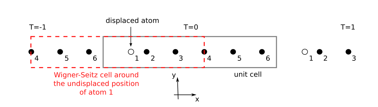
Fig. 152 A 1D chain with 6 atoms per unit cell with atom 1 being displaced. The periodically-repeated atoms to the left (\(T=-1\)) and to the right (\(T=1\)) are indicated. The Wigner-Seitz cell centered at the undisplaced position of atom 1 is drawn red / dashed.

All atoms are at their equilibrium positions, besides atom 1 which is displaced along the \(x\) direction. The force on atom 5, for example, can be regarded as “repulsive” due to the displacement of atom 1 in the unit cell with translation \(T=0\) along the \(x\)-axis. However, there is also an “attractive” contribution from the image of the displaced atom 1 in the unit cell with translation \(T=1\). To decompose the two contributions we construct a Wigner-Seitz cell centered at the undisplaced position of atom 1 and check the distance to the nearest neighbor representations of atom 5. The representation of atom 5 inside the cell at \(T=0\) is not part of the Wigner-Seitz cell, and thus this contribution is neglected. In contrast, the representation of atom 5 at \(T=-1\) is inside the Wigner-Seitz cell and we keep this contribution. If an atom is at the face (like atom 4), the edge or a vertex of the Wigner-Seitz cell, the force is included weighted by the inverse multiplicity of this Wigner-Seitz grid point. This construction is repeated for all atoms inside the unit cell. In this way it is possible to approximately calculate the entries of the DynamicalMatrix for all repetitions of the cell from \(T = -1\) to \(T = 1\) and thereby get the dispersion, by only calculating the forces in a single unit cell.

Note

The Wigner-Seitz construction ensures that the phonon spectrum at the \(\Gamma\)-point is preserved. Hence, a separate \(\Gamma\)-point calculation is not necessary.

Notes for polar phonon splitting

In polar materials the covalency will change during ionic displacements since a macroscopic electric field is generated. This gives rise to an extra force constant term in the dynamical matrix. The full dynamical matrix is \(\mathbf{D}(\mathbf{q}) = \mathbf{D}^{FC}(\mathbf{q}) + \mathbf{D}^{NA}(\mathbf{q})\). Here \(\mathbf{D}^{FC}(\mathbf{q})\) is the usual force constant dynamical matrix discussed above and the second term \(\mathbf{D}^{NA}(\mathbf{q})\) is due to polar phonon interaction. The non-analytic (NA) contribution from the macroscopic field to the dynamical matrix is:

\[\mathbf{D}^{NA}_{i\mu j\nu}(\mathbf{q}) = \frac{e}{\epsilon_0 \Omega \sqrt{M_iM_j}}\frac{[\mathbf{Z}(i)\cdot \hat{\mathbf{q}}]_{\mu} [\mathbf{Z}(j)\cdot \hat{\mathbf{q}}]_{\nu}}{\hat{\mathbf{q}}\epsilon^{\infty} \hat{\mathbf{q}}} \,.\]

Here \(\mathbf{Z}(i)\) is the Born effective charge tensor (a matrix for atom \(i\)), \(\hat{\mathbf{q}}=\mathbf{q}/|\mathbf{q}|\) is a unit vector, \(M_i\) is the mass of atom \(i\), \(\Omega\) is the unit cell volume, \(e\) is the electron charge and \(\epsilon_{0}\) is the vacuum permittivity. The term non-analytical refers to the fact that it approaches different values from different \(\mathbf{q}\)-space directions as \(q\rightarrow 0\). It is obtained from the BornEffectiveCharge calculation and the high-frequency dielectric tensor \(\epsilon^{\infty}\) obtained from the OpticalSpectrum.

The Dynamical Matrix study object will automatically include a calculation of the BornEffectiveCharges and OpticalSpectrum or it can be given by the user from an existing calculation. To include polar phonon splitting in the dynamical matrix study object one has to give PolarPhonon_splitting_parameters as input:

dynamical_matrix = DynamicalMatrix(
    configuration,
    filename='DynamicalMatrix.hdf5',
    object_id='dynamical_matrix',
    repetitions=(1,5,3),
    polar_phonon_splitting_parameters=pps_parameters,
)
dynamical_matrix.update()

Here the polar polar_phonon_splitting_parameters is a container of polar phonon splitting parameters. It can either be setup by defaults

pps_parameters = PolarPhononSplittingParameters()

Or it can be set with specific user-defined variables for optical spectrum and Born effective charges.

pps_parameters = PolarPhononSplittingParameters(
    kpoints=MonkhorstPackGrid(25, 25, 25),
    broadening=0.1 * eV,
    bands_below_fermi_level=35,
    bands_above_fermi_level=35,
    kpoints_a=MonkhorstPackGrid(19, 9, 9),
    kpoints_b=MonkhorstPackGrid(9, 19, 9),
    kpoints_c=MonkhorstPackGrid(9, 9, 19),
    atomic_displacement=0.01 * Ang,
)

Finally it can be defined from existing calculations of the OpticalSpectrum and BornEffectiveCharge:

pps_parameters = PolarPhononSplittingParameters(
    optical_spectrum=optical_spectrum,
    born_effective_charge=born_effective_charge,
)

This last option enables the combination of force constants obtained from a classical calculator with polar phonon splitting obtained from ATK-DFT.

Notes for internal coordinates

For molecules, it can be beneficial to shift the dynamical matrix into an internal coordinate basis when conducting studies of or including the vibrational modes of a MoleculeConfiguration. A (potentially) redundant internal coordinate basis is generated by converting the bond connectivity of the molecule into unique stretch, bend, and dihedral internal coordinates, from which a non-redundant set of \(3N-6\) (in the general case) linear combinations of internal coordinates are derived. This scheme thus allows a non-redundant description of the vibrational modes and results in the same number of vibrational modes as the number of degrees of freedom in the molecule.

The internal coordinate scheme assumes that the bond connectivity of the system connects all atoms in the configuration, so that at least \(3N-6\) unique internal coordinates are generated. If fewer bonds are present, or if only a smaller number of bonds can be automatically discovered, the internal coordinate scheme will yield fewer vibrational modes than the degrees of freedom in the molecule. The use_internal_coordinates argument should therefore only be activated when all bonds in a molecule can be automatically discovered with the findBonds() method of a MoleculeConfiguration object or are set manually on the configuration. This can be done from the Builder or in scripting. Alternatively, a bond_list argument can be passed to a DynamicalMatrix object with the desired bonding behaviour, in which all atom indices are included and interconnected in a single molecule fragment.