NVTBussiDonadioParrinello

class NVTBussiDonadioParrinello(initial_velocity=None, time_step=None, reservoir_temperature=None, heating_rate=None, thermostat_timescale=None, random_seed=None)

The NVT Bussi-Donadio-Parrinelllo thermostat.

Parameters:

• initial_velocity (ConfigurationVelocities | ZeroVelocities | MaxwellBoltzmannDistribution) – A class that implements a distribution of initial velocities for the particles in the MD simulation.
  Default: MaxwellBoltzmannDistribution

• time_step (PhysicalQuantity of type time) – The time-step interval used in the MD simulation.
  Default: 1 * fs

• reservoir_temperature (PhysicalQuantity of type temperature | list) – The reservoir temperature in the simulation. The temperature can be given as a single temperature value for the entire system, or as a list of 2-tuples of str and PhysicalQuantity of type temperature, applying local thermostats to the tagged groups of atoms. E.g. [('group1', 280.0 * Kelvin), ('group2', 320.0 * Kelvin)].
  Default: 300.0 * Kelvin

• heating_rate (PhysicalQuantity of type temperature/time | None) – The heating rate of the target temperature. A value of None disables the heating of the system.
  Default: 0.0 * Kelvin / fs

• thermostat_timescale (PhysicalQuantity of type time) – The time constant for temperature coupling.
  Default: 100.0 * fs

• random_seed (int) – The seed for the random generator providing the stochastic part of the velocity scaling. Must be between 0 and 2**32.
  Default: The default random seed

kineticEnergy(configuration)

Parameters:

configuration (DistributedConfiguration) – The current configuration to calculate the kinetic energy of.

Returns:

The kinetic energy of the current configuration.

Return type:

PhysicalQuantity of type energy

thermostats()

Returns:

The list of thermostats.

Return type:

list

timeStep()

Returns:

The time step.

Return type:

PhysicalQuantity of type time

uniqueString()

Return a unique string representing the state of the object.

Usage Example

Perform a molecular dynamics run of 50 steps on FCC Si, using the Bussi-Donadio-Parrinello thermostat:

# Set up configuration
bulk_configuration = BulkConfiguration(
    bravais_lattice=FaceCenteredCubic(5.4306*Angstrom),
    elements=[Silicon, Silicon],
    fractional_coordinates=[[0.0, 0.0, 0.0], [0.25, 0.25, 0.25]]
    )

# Set calculator
calculator = TremoloXCalculator(parameters=Tersoff_Si_1988b())
bulk_configuration.setCalculator(calculator)

# Set up MD method
method = NVTBussiDonadioParrinello(
    time_step=1*femtoSecond,
    reservoir_temperature=300*Kelvin,
    thermostat_timescale=100*femtoSecond,
    heating_rate=0*Kelvin/picoSecond,
    initial_velocity=None
)

# Run MD simulation
md_trajectory = MolecularDynamics(
    bulk_configuration,
    constraints=[],
    trajectory_filename='trajectory.nc',
    steps=50,
    log_interval=10,
    method=method
)

nvtbussidonadioparrinello.py

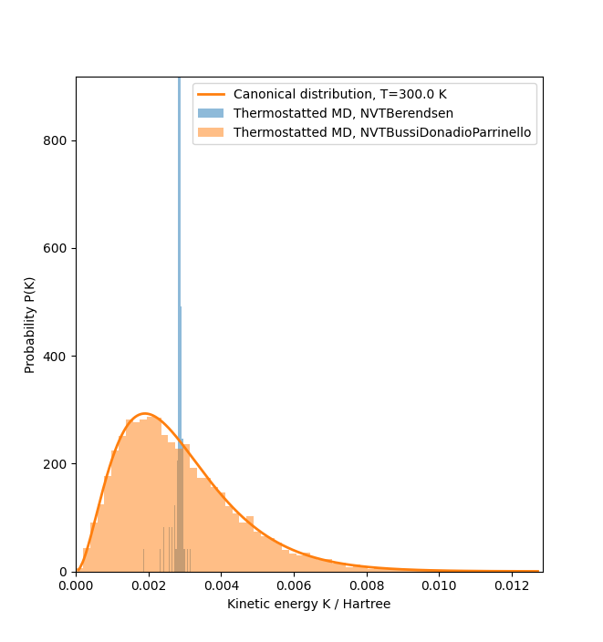
The script below demonstrates that the Bussi-Donadio-Parrinello produces a NVT ensemble, while the Berendsen thermostat fails to do so. The histogram of the kinetic energies from a long molecular dynamics trajectory is compared with the expected canonical distribution for the kinetic energy.

The analytical expression for the canonical equilibrium distribution of the kinetic energy \(K\) at temperature \(T\) is given by

\[P(K) dK = \frac{\beta^{N_f/2}}{\Gamma(N_f/2)} K^{N_f/2-1} \exp(-\beta K) dK\]

where \(\beta = 1/(k_B T)\) and \(N_f\) is the number of degrees of freedom.

import matplotlib.pyplot as plt

# Increase the number of MD steps to converge the histograms.
STEPS = 5000

plt.xlabel("Kinetic energy K / Hartree")
plt.ylabel("Probability P(K)")

# Set up configuration
bulk_configuration = BulkConfiguration(
    bravais_lattice=FaceCenteredCubic(5.4306*Angstrom),
    elements=[Silicon, Silicon],
    fractional_coordinates=[[0.0, 0.0, 0.0], [0.25, 0.25, 0.25]]
    )

# Set calculator
calculator = TremoloXCalculator(parameters=Tersoff_Si_1988b())
bulk_configuration.setCalculator(calculator)

# Run MD simulations with each thermostat.
for thermostat_class in NVTBerendsen, NVTBussiDonadioParrinello:
    # Set up MD method
    method = thermostat_class(
        time_step=1*femtoSecond,
        reservoir_temperature=300*Kelvin,
        thermostat_timescale=100*femtoSecond,
        heating_rate=0*Kelvin/picoSecond,
        initial_velocity=ZeroVelocities(),
    )

    # Run long MD simulation
    md_trajectory = MolecularDynamics(
        bulk_configuration,
        constraints=[],
        trajectory_filename='trajectory.hdf5',
        steps=STEPS,
        log_interval=50,
        method=method
    )

    # Choose color and label for thermostat
    color = next(plt.gca()._get_lines.prop_cycler)["color"]
    label = thermostat_class.__name__

    # Kinetic energy distribution from samples in MD trajectory.
    temperatures = numpy.unique(md_trajectory.reservoirTemperatures())
    assert len(temperatures) == 1, 'Reservoir temperature should not change during MD run.'
    temperature = temperatures[0]
    beta = (1.0/(boltzmann_constant * temperature)).inUnitsOf(Hartree**(-1))
    ekin = md_trajectory.kineticEnergies().inUnitsOf(Hartree)

    # Plot histogram of kinetic energies
    plt.hist(
        ekin,
        bins='auto', alpha=0.5,
        color=color, stacked=True, density=True, label=f'Thermostatted MD, {label}'
    )

# Find number of degrees of freedom
n = bulk_configuration.numberOfAtoms()
Nf = 3*n

# To avoid overflows reorganize the expression for P(K),
# so the logs of large quantities cancel before exponentiating.
def logGamma(x):
    """ Expansion of log(Gamma(x)) for large x """
    lG = (x-0.5) * numpy.log(x) - x + 0.5*numpy.log(2.0*numpy.pi)
    return lG

# For K=0.0, log(beta^*K) gives inf.
ekin = ekin[ekin > 0.0]
ekin.sort()

probability_canonical = numpy.exp(
    Nf/2.0 * numpy.log(beta*ekin) - beta*ekin - logGamma(Nf/2.0)
) / ekin

# Plot canonical distribution
plt.plot(
    ekin, probability_canonical,
    color=color, lw=2, label=f'Canonical distribution, T={temperature.inUnitsOf(Kelvin)} K'
)

plt.legend()
plt.show()

kinetic_energy_distribution.py

Notes

• The Bussi-Donadio-Parrinello thermostat [1], [2] is a stochastic variant of the Berendsen thermostat. However, unlike the Berendsen thermostat it correctly samples the canonical NVT-ensemble. The factor for scaling the velocities is a random number, which is generated in such a way as to produce the canonical equilibrium distribution for the kinetic energy.

• You can specify one or more thermostats acting on tagged sub-groups of atoms of the configuration, by giving a list of (tag-name, temperature)-tuples instead of a single, global reservoir_temperature value.

• If a non-zero heating_rate is specified, the reservoir temperature will be changed linearly during the simulation, according to the specified heating rate.

[1]

Giovanni Bussi, Davide Donadio, and Michele Parrinello. Canonical sampling through velocity rescaling. Journal of Chemical Physics, 126(1):014101, 2007. doi:10.1063/1.2408420.

[2]

Giovanni Bussi and Michele Parrinello. Stochastic thermostats: comparison of local and global schemes. Computer Physics Communications, 179(1-3):26–29, 2008. doi:10.1016/j.cpc.2008.01.006.