Band Structure of a SiC Crystal
You will here learn how to use QuantumATK for calculating the band structure and other properties of a SiC crystal. We shall not discuss the science of such a calculation much; the purpose of the tutorial is to show how to operate QuantumATK, specifically how to set up simple calculations and visualize the results.
Workflow

Build SiC Crystal
Start QuantumATK and create a new project with the title you prefer, e.g. SiC_study. Then open the project.
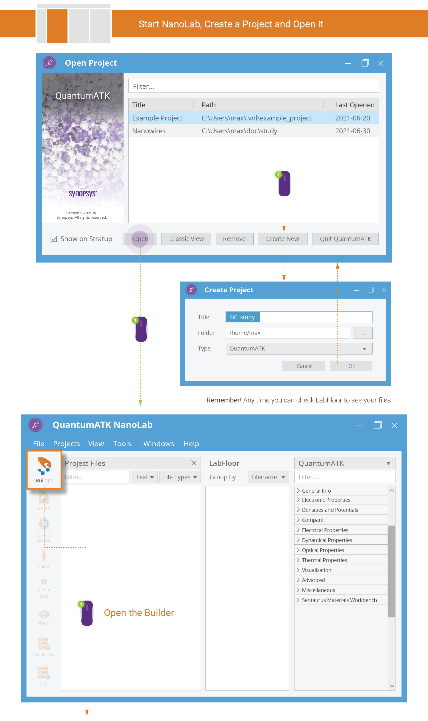
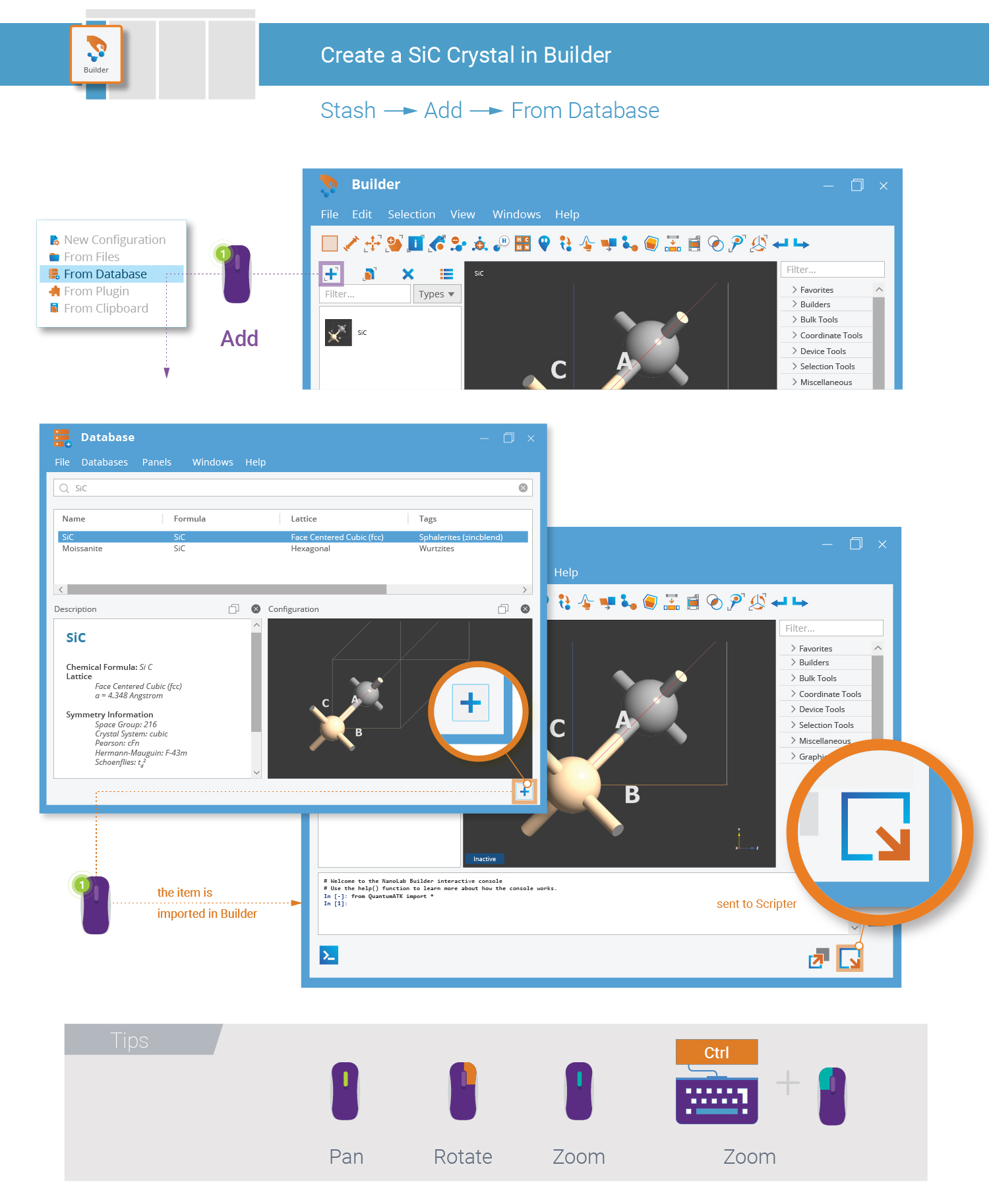
Use the Database plugin to quickly build the SiC bulk configuration.
Tip
Several QuantumATK tools contain a 3D preview of the currently active configuration. Use the right mouse button to rotate the 3D view, use the scroll wheel to zoom (or hold down Ctrl and right mouse button and move the mouse), and press the scroll wheel and move the mouse to pan the camera (or hold down Shift and the right mouse button and move the mouse).
Setup QuantumATK Calculation
You are now ready to setup an QuantumATK Python script that calculates the electronic
ground state of the SiC crystal followed by analysis of the band structure and
electron density. This is what the  Script Generator
is used for (“Scripter” for short).
Script Generator
is used for (“Scripter” for short).
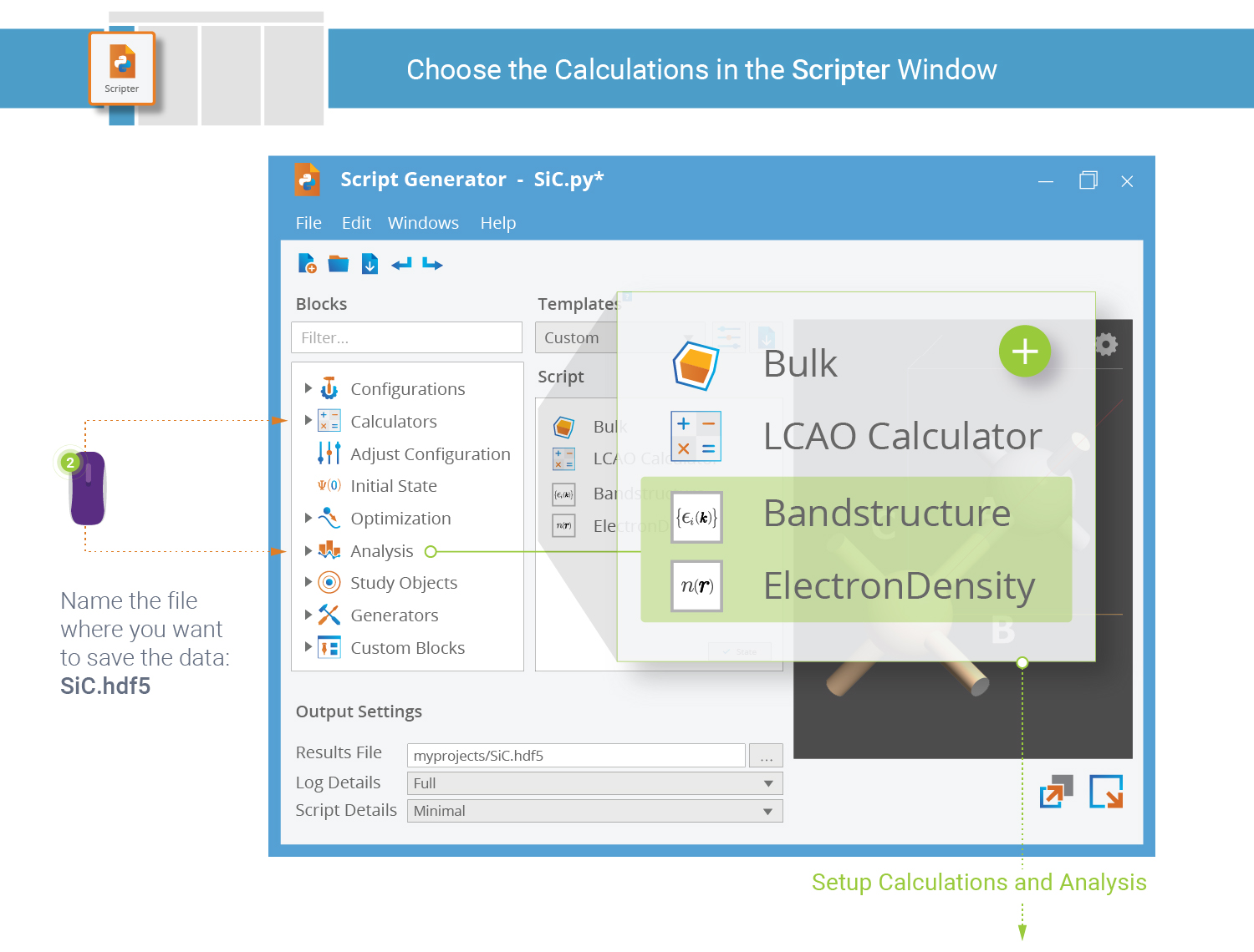
Transfer the SiC crystal from the Builder to the Scripter by clicking the
Send to icon  in the lower-right corner of the Builder
window, and select “Script Generator” from the pop-up menu. The Scripter
appears and the Builder window is automatically minimized.
in the lower-right corner of the Builder
window, and select “Script Generator” from the pop-up menu. The Scripter
appears and the Builder window is automatically minimized.
The script already contains the SiC bulk configuration. Add the Calculator block and two Analysis blocks.
New Calculator Block
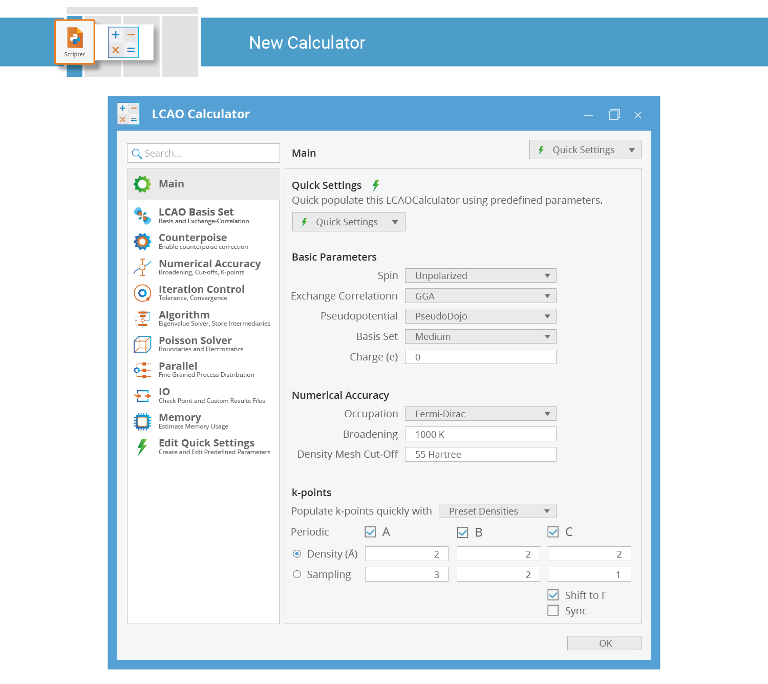
The calculator computes the ground state of the SiC crystal. It contains a wide range of settings, all of which have sensible default values. However, you will most often need to change at least a few of them in order to make the calculation match your scientific goals.
Double-click the New Calculator block when you wish to edit it:
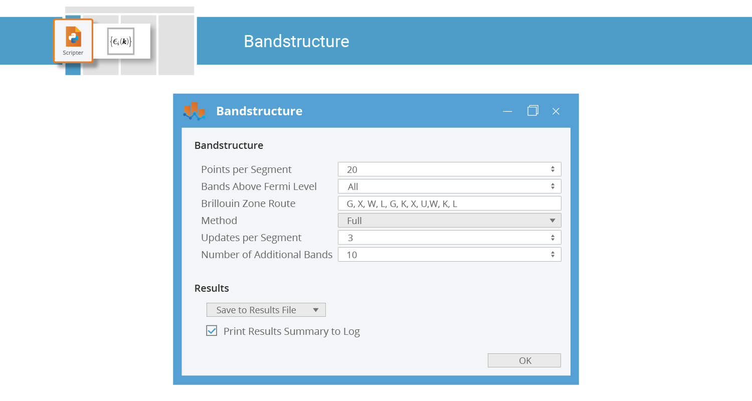
Analysis Blocks
The Bandstructure and ElectronDensity blocks perform post-SCF analysis. Double-click the Bandstructure block to increase the Brillouin zone sampling:
Saving the Script
The QuantumATK script is now done, and it is good practice to immediately save it. Use the File menu in the Script Generator, or the keyboard shortcut Ctrl+Shift+S.
Run Calculations
You need to run the QuantumATK Python script in order to execute the calculations. This can be done from a terminal:
atkpython example.py > example.log
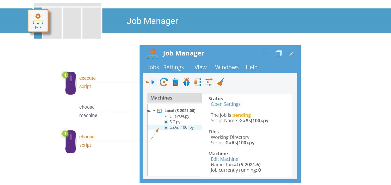
A very convenient alternative is to use the  Job Manager
to run the script directly from inside QuantumATK:
Job Manager
to run the script directly from inside QuantumATK:
Click the
in the lower-right corner of the Script Generator, and select “Job Manager” from the menu.The “Save As” dialog appears, prompting you to make sure the script is saved, followed by the Job Manager window and the “Select Machine” dialog.
Choose a “Local” machine type, and click OK. The QuantumATK Python script is added to the job queue of the chosen machine.
Select your script and click the
 button to start
executing the calculation.
button to start
executing the calculation.
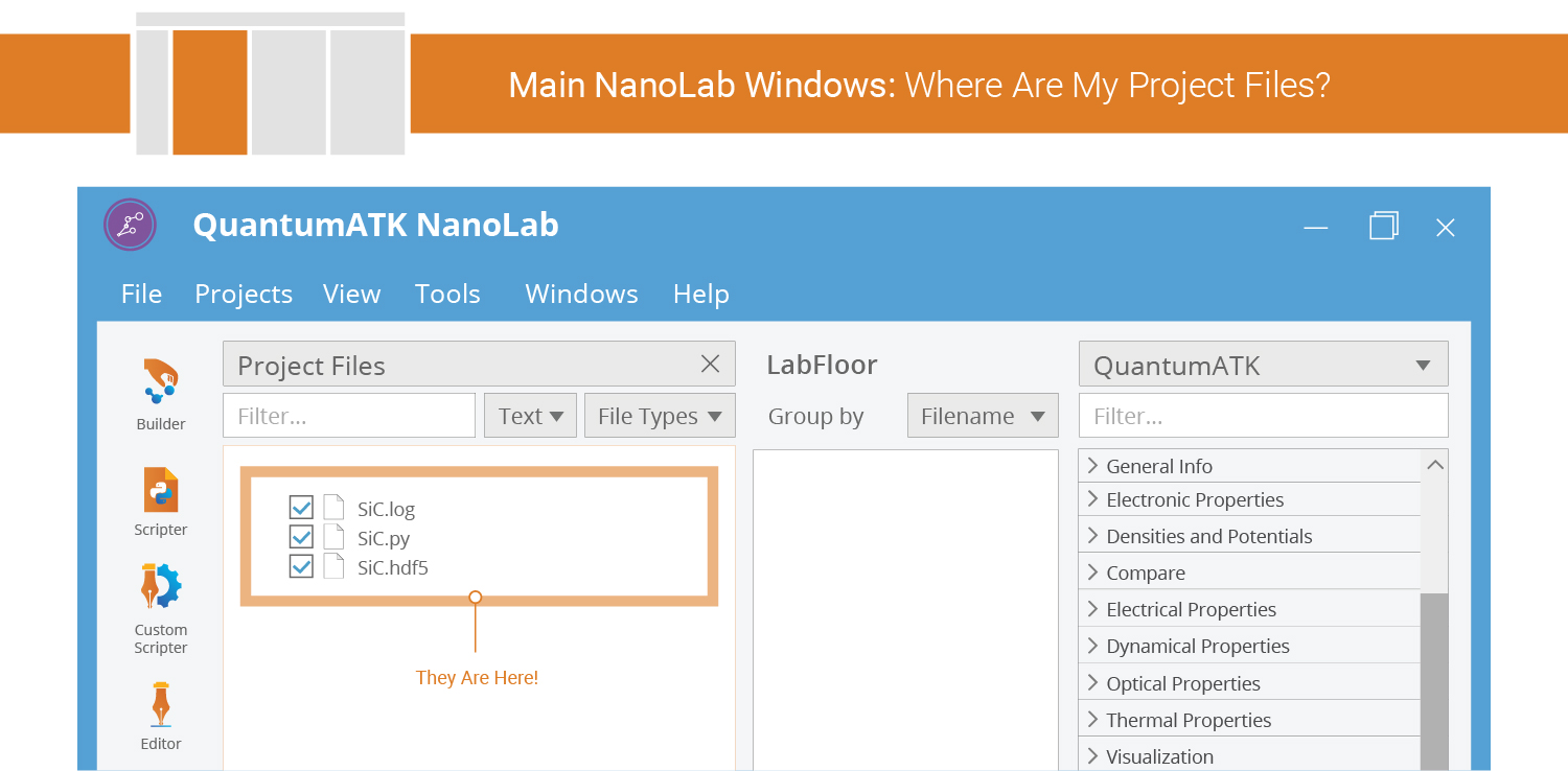
Calculation Output
Any output (data, log, etc.) should appear in the Project Files list.
New .hdf5 files are automatically scanned and their contents displayed
on the LabFloor.
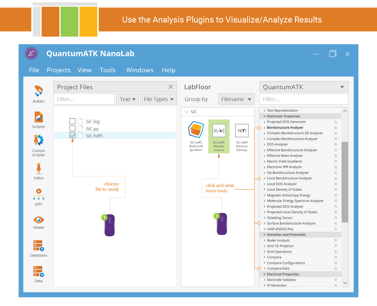
Analyze and Visualize Results
The calculation has now finished and you are ready to study the results. To this end, return to the QuantumATK main window to select one of the saved data items and see the list of applicable analysis plugins.
Tip
Use the keyboard shortcut Alt+W to activate the Windows menu, which allows you to easily switch between different QuantumATK windows.
Band Structure
The HDF5 data file is SiC.hdf5. Make sure the file is ticked in the
Project Files list in order to see its contents on the LabFloor. You may have
to expand the LabFloor item. Select the band structure item and
click the Bandstructure Analyzer in the right-hand Panel Bar.
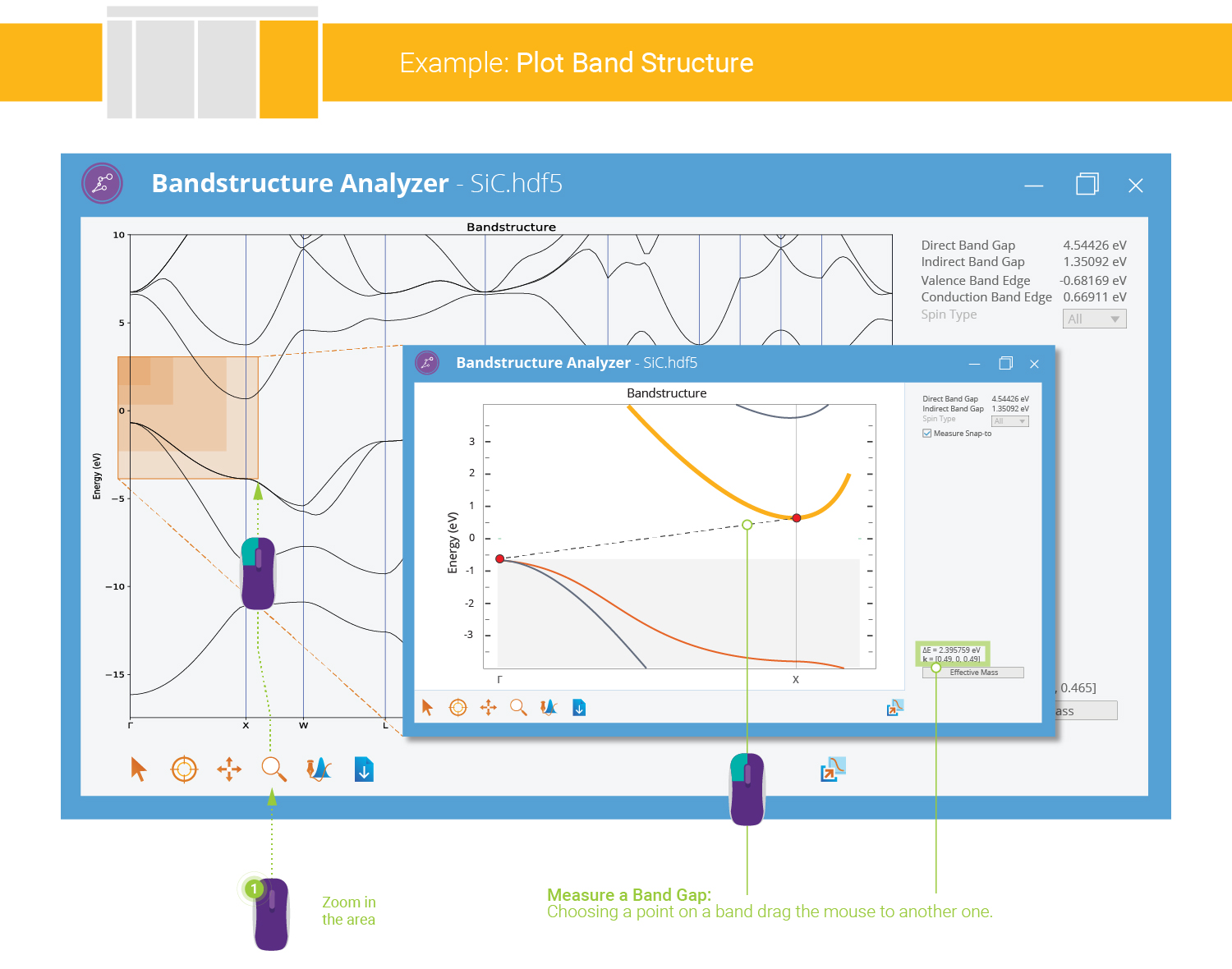
both the direct and indirect band gaps are given by the analyzer. In general it is easy to measure both the direct and indirect band gaps with NanoLab. In the present case we measure the indirect gap between the Γ and X points in reciprocal space:
Click the
 icon to activate the Zoom to rectangle function,
and zoom into the relevant part of the band structure.
icon to activate the Zoom to rectangle function,
and zoom into the relevant part of the band structure.Deactivate Zoom, and use the mouse to measure the indirect band gap.
Electron Density
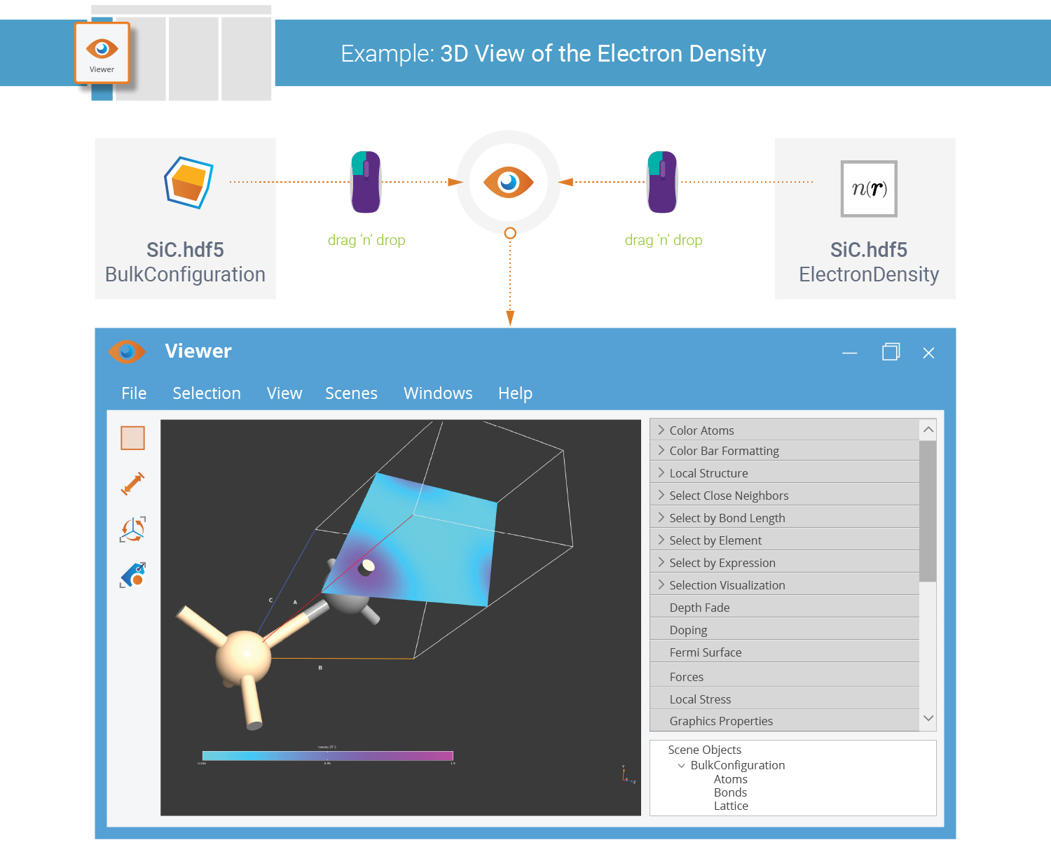
The  Viewer is used to visualize configurations and also
data that is represented on 3D grids. You can visualize the SiC unit cell
and the self-consistent electron density in a single view:
Viewer is used to visualize configurations and also
data that is represented on 3D grids. You can visualize the SiC unit cell
and the self-consistent electron density in a single view:
Drop the SiC bulk configuration on the Viewer.
Select on the LabFloor the ElectronDensity item,
 ,
and just drop it on the SiC visualization. Choose a cut-plane representation.
,
and just drop it on the SiC visualization. Choose a cut-plane representation.
A default visualization style is used. Use the Properties tool in the Viewer panel bar to adjust the visualization settings as you prefer.
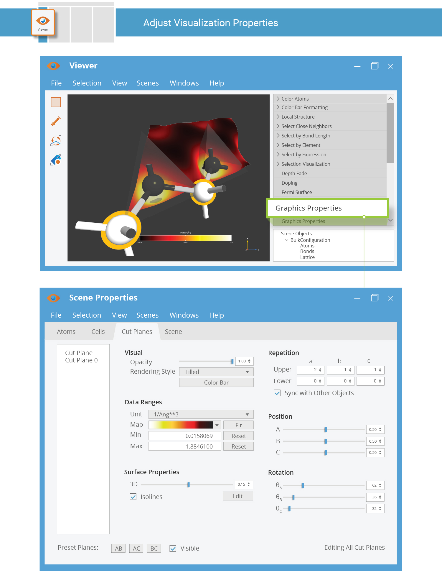
Tip
To export the visualization as an image, use the right mouse button menu Export image.
Additional Analysis
Suppose you now want to perform some additional analysis of the SiC crystal, e.g. compute the electronic Density Of States (DOS). This is easily done by creating and running a new QuantumATK Python script that uses the Analysis from File functionality.
Simply open the Script Generator and create the
script as illustrated below. In the Analysis from File block, load the saved
HDF5 file Sic.hdf5. The widget should automatically detect and select
the BulkConfiguration. Lastly, change the default output filename to
SiC.hdf5 and save the script as SiC_analysis.py.
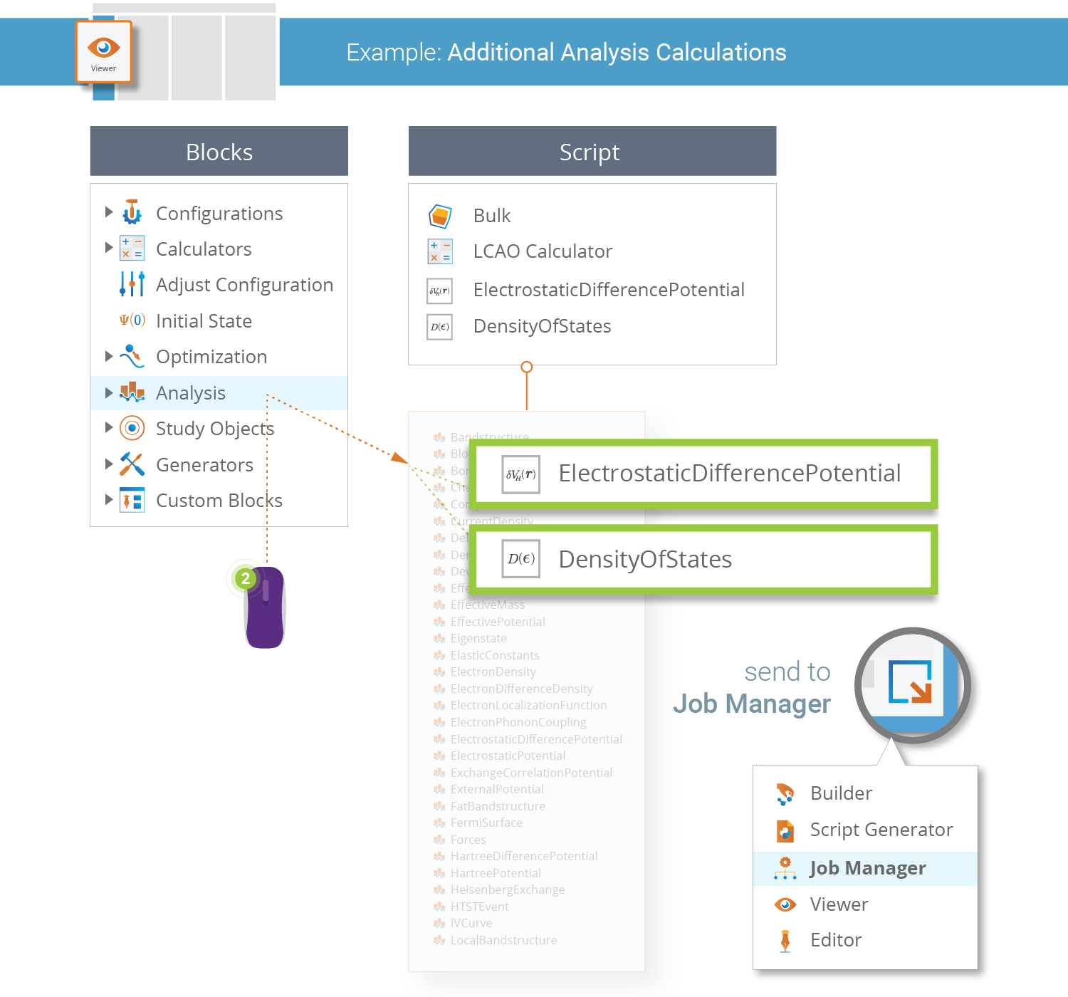
What happens in the QuantumATK Python script you just made is this:
The self-consistent electronic structure of the SiC bulk was previously calculated, so here we simply read that state using Analysis from File.
Two different post-SCF analyses are then performed; first the electrostatic difference potential is computed, and then the density of states. Both data items are appended to the existing data file
SiC.hdf5.
Send the script to the Job Manager and run the calculations.
Plotting the Density of States
The SiC density of states is now easily plotted; select the DOS object on the LabFloor,
 , and click the 2D Plot plugin in the
right-hand Panel Bar. You should now see a plot of the computed DOS vs. electron energy
eigenvalue (referenced to the Fermi level). Use the mouse to zoom in on the plot if needed.
, and click the 2D Plot plugin in the
right-hand Panel Bar. You should now see a plot of the computed DOS vs. electron energy
eigenvalue (referenced to the Fermi level). Use the mouse to zoom in on the plot if needed.
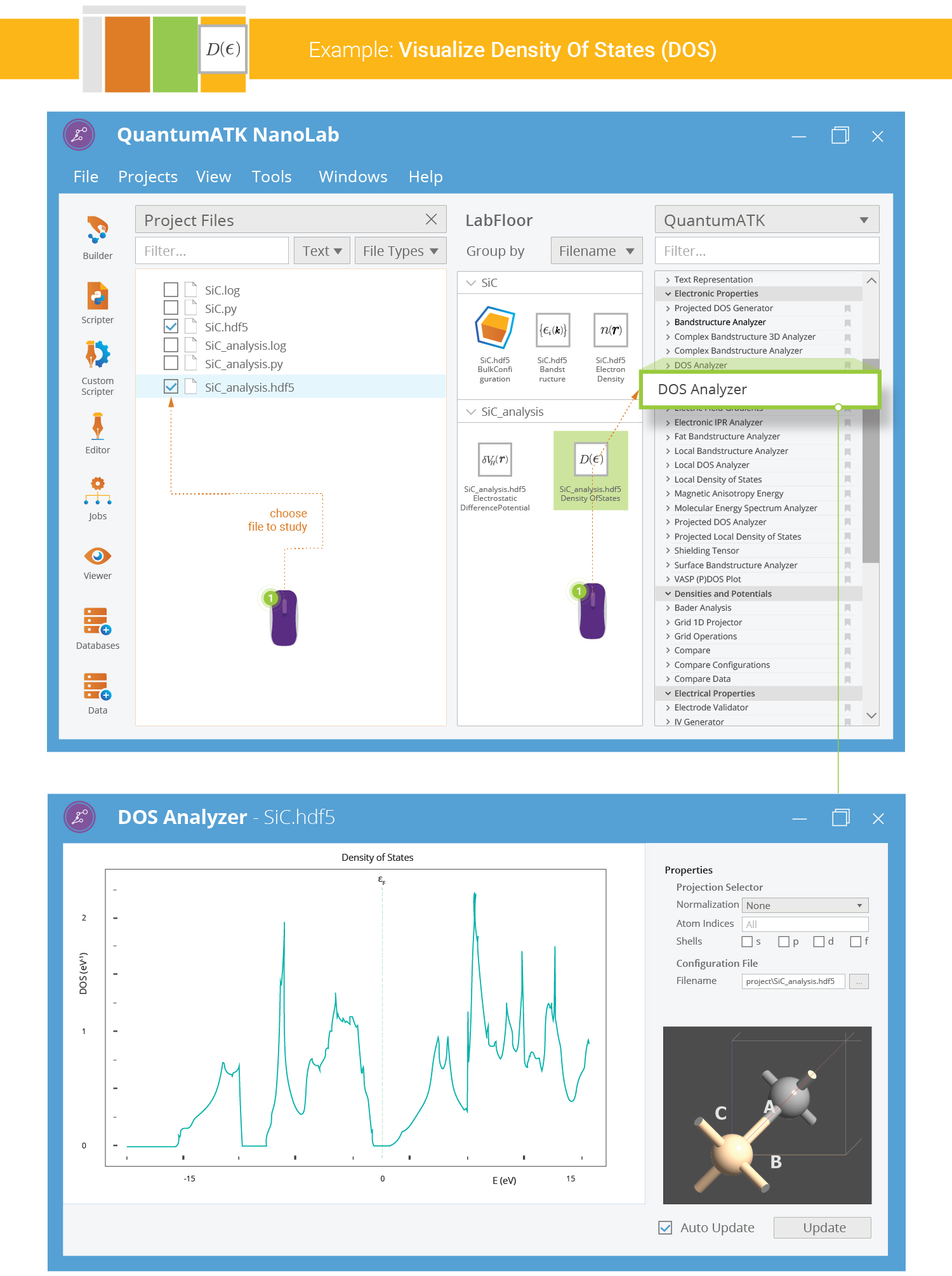
You can also plot the projected DOS using the Projection selector: Select the carbon atom (index 1) and tick only the p-shell in order to see the PDOS corresponding to the p-orbital of the C atom.
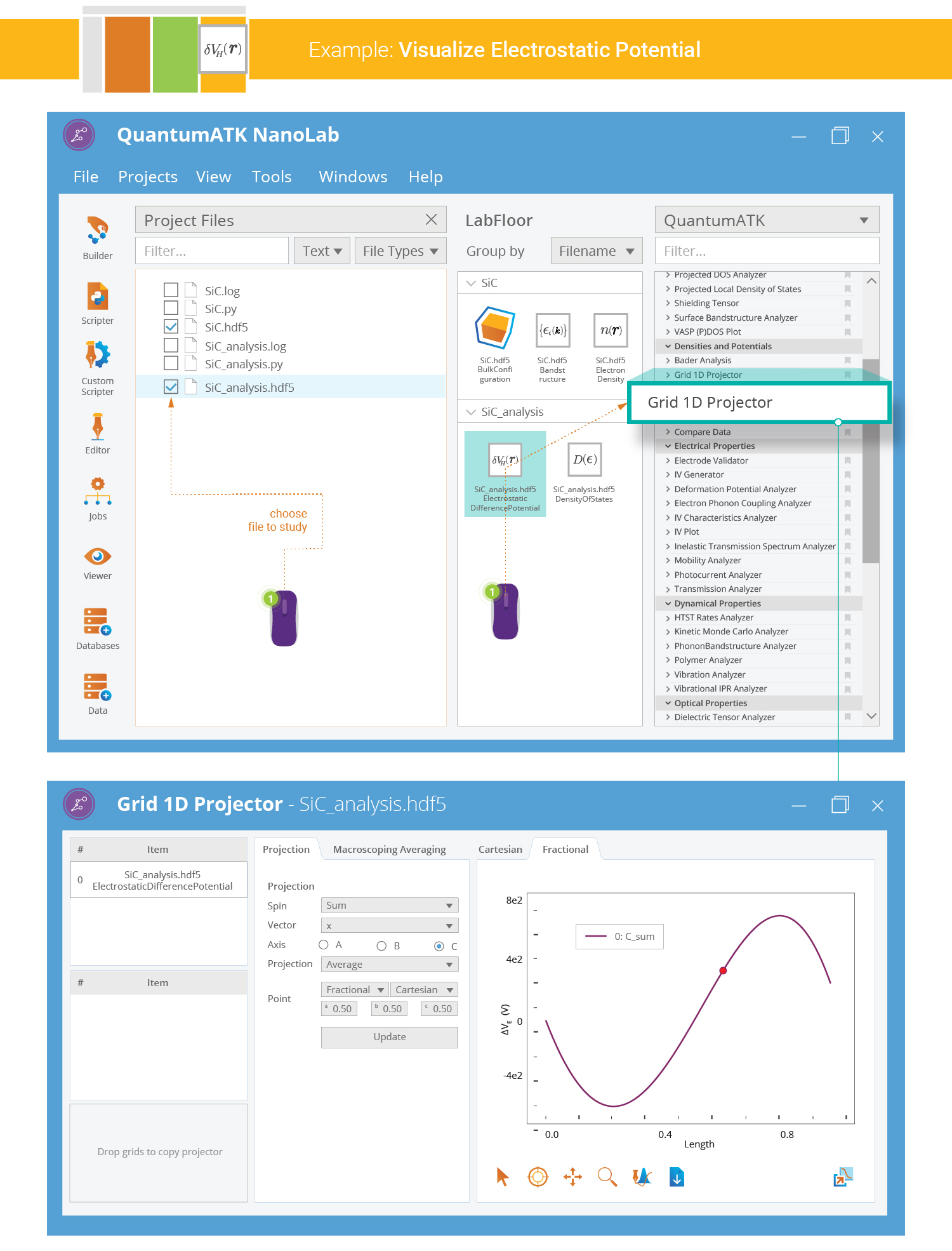
1D Projection of the Electrostatic Potential
The electrostatic difference potential (EDP) is represented on a 3D grid, and you could visualize it as an isosurface or a cut plane in the 3D Viewer. However, QuantumATK also offers a very convenient tool for creating 1D projections of 3-dimensional grid data - the 1D Projector:
Select the EDP data item on the LabFloor,
 ,
and click the 1D Projector plugin.
,
and click the 1D Projector plugin.Choose “C” as the projection axis and “Sum” as the projection type.
Then click Add line to produce the plot.
Note
The plot above shows the summed EDP along the C-axis of the SiC bulk configuration, i.e. summed in the AB plane for each value of C. You can also choose to average the grid values instead of summing them. Use the “Through point” projection type to avoid summing or averaging the grid values altogether.