Transmission spectrum of perfect sheets of graphene and MoS2
Transmission spectrum of perfect sheets of graphene and MoS2
In this tutorial, you will learn how to calculate the transmission spectrum of graphene and MoS2. The focus of this tutorials is on what parameters to choose, what to calculate, and what to think about, rather than all the details of “how”.
In QuantumATK it is possible to compute the transmission spectrum of a perfect periodic system in a simple way, which doesn’t require the more detailed setup of a device configuration, with electrodes, electrode extensions, and scattering region, which normally is necessary when the system is not perfect. In this example you will look at how to compute the transmission spectrum of a perfect, periodic 2D sheet. The first example will be graphene - since it is well-known and popular - and then let’s consider MoS2 which has a more complicated unit cell.
For a perfectly periodic structure the transmission spectrum is in principle just a sum over the available modes in the band structure at each energy. In a 1D system this is manageable by hand, but already for a 2D system one has to consider how to sample the Brillouin zone properly, both for the electronic structure and the transmission spectrum itself.
The focus of this tutorials is on “what” - what parameters to choose, what to calculate, what to think about, rather than all the details of “how”. It will thus be assumed that you have some rudimentary experience using QuantumATK, as obtained from going through some of the Basic QuantumATK Tutorial.
One basic thing to note is that QuantumATK uses a similar methodology to compute the transmission spectrum as the complex band structure. Therefore the same rule applies: the unit cell must be “electrode-like”, meaning that the A and B vectors must both be perpendicular to the C vector, which should be parallel to Z, and which defines the direction in which we compute the transmission (not all materials are isotropic!).
It is however not necessary to repeat the cell in the C-direction; you can always leave it as the smallest possible cell. QuantumATK will, however, internally repeat enough to include all relevant interactions.
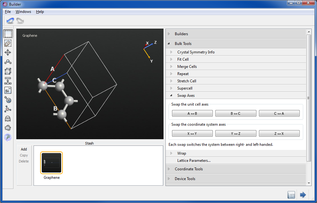
Now let us apply this to graphene, and your first task is thus to convert the hexagonal unit cell to some thing orthorhombic. This is easily achieved in the Builder:
Click Add>Add From Database…, locate graphene and add the structure to the stash.
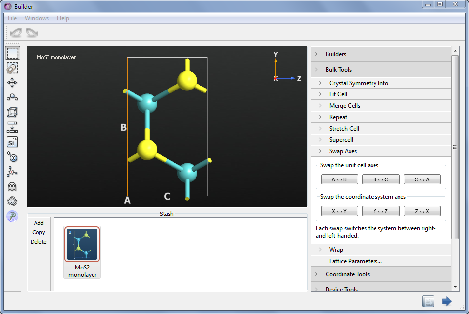
Open Bulk Tools>Supercell and enter the values as shown in the picture below. Then press Transform.
You now have an orthogonal cell, but the Z direction is pointing out of the graphene plane; it should lie in the plane. Therefore, open Bulk Tools>Swap Axes and interchance the A and C axes. This brings C into the plane, however the cell is now left-handed, and moreover C is not pointing along Z but along X. This is remedied by a second switch, of Z and X. You now have a proper cell for the transmission spectrum calculation, with a Z/C-axis pointing along the zigzag direction (however, in graphene, the transmission is isotropic, so you would get the same result along the armchair direction).
In this example you will use a simple tight-binding model to make the calculations fast, more specifically a 3rd nearest neighbor single pi-band model. For “simple” graphene this provides an excellent band structure, which is all we really need for the transmission spectrum.
Graphene is however slightly tricky because it’s hard to know how many k-points you need to get converged results; the peculiar band structure around the K point makes it important to include this point - or several points around it - to get accurate values. The general rule is that you need an odd integer multiple of 3 (although some care needs to be taken with supercells). With the simple nearest-neighbor tight-binding model, the band structure is however essentially encoded into the method, and you actually don’t need more than 3 k-points in the B and C directions. (For DFT, you will need at least 9 points, and preferably more.)
To set these parameters:
In the Script Generator, double-click New Calculator to insert a calculator block.
Open it, and select “ATK-SE: Slater-Koster”.
Set the k-point sampling to 3 points in B and 3 points in C.
Go to the “Slater-Koster basis set” section and choose the Hanock.C basis set in the “Predefined” list.
Close the New Calculator.
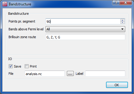
To verify that you do obtain a good band structure, insert a Analysis>Bandstructure block; double-click it and set the number of points to 90 (so that you hit the K point, which in this geometry lies on the G-Z path). Also add X, G to the path, so that the essential parts of the 2D zone are covered.
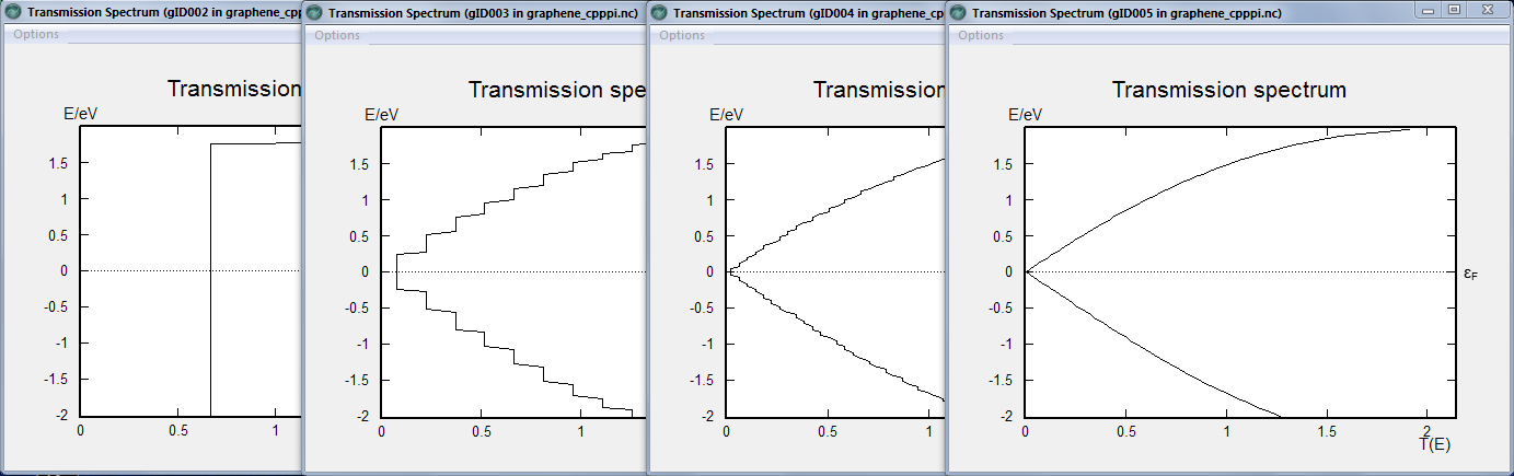
For the transmission spectrum, you need to sample the Brillouin zone very densely to get an accurate curve. To illustrate this, you will compute the transmission for a few different value of the k-point sampling, and compare.
Insert a Analysis>TransmissionSpectrum block 4 times. Double-click each one, and set a different number of k-points in the B direction (note that there is no need to set them in A, and no option to set them in C) in each one, as follows: 3, 27, 99, 601.
Finally:
Set the name of the output file.
Save the script.
Send the calculation to the Job Manager.
The electronic structure part will literally take seconds, and the transmission spectra are also very fast to compute; the whole script should finish in well under a minute.
You can now open the four different transmission spectra and inspect the differences. Clearly, using 3 and 27 k-points does not give any useful results, but even at 99 k-points the curve is still very jagged compared to the “converged” result at 601 points.
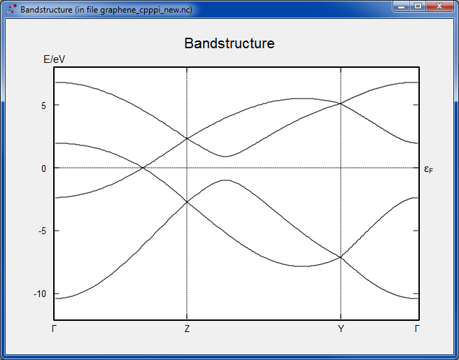
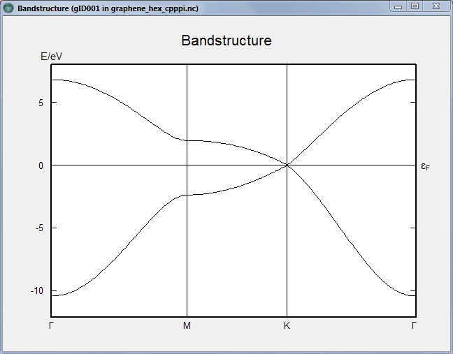
Checking the band structure, you see a perfect shape of the bands close to the Fermi level, as expected from the purpose of the parameterization used. The K point is clearly visible, although it appears without a label inbetween Γ and Z since in this case, as mentioned above, we now have a supercell and so the Brillouin zone is folded.
It is left as an exercise to perform the band structure calculation using the same basis set, for the simple hexagonal graphene unit cell. The result is shown below. Don’t forget that if you just take graphene from the database, the axes are oriented such that the k-point sampling needs to be applied in the A/B plane.
The second example will be on a material that is similar to graphene, but also very different. MoS2 or molybdenite is a crystal which also has a hexagonal unit cell, reminiscent of graphite, although the basis is more complex, with Mo and two S atoms. It has been found molybdenite can also form monoatomic layers, but unlike graphene it has a finite band gap.
Many details of the calculation for MoS2 will be left as an exercise - the steps are very similar, even if there are some notable differences in terms of parameter choices that are worthwhile commenting on.
ATK contains a Slater-Koster model (DFTB) for Mo-S already, contained in the (admittedly experimental) CP2K set. It’s a non-selfconsistent model, but as we will see it compares fairly well to DFT, at least for the conduction band and in general in the areas around the band edges.
Send the structure to the Script Generator.
Insert a New Calculator block and open it.
Select the ATK-SE: Slater-Koster calculator, and set the k-point sampling to 1x3x3, as for graphene. (Testing shows that there is a negligible difference in the band structure compared to 1x27x27 k-points also in this case.)
Under “Slater-Koster basis set”, you will notice that there is only one choice in the list of built-in (predefined) sets, viz. the CP2K model.
As for graphene, insert a Bandstructure block and again change the number of points (90) and route (G-Z-Y-G).
This time you can pretty much guess that just as for graphene, you will need the 601 k-points to get proper results, so just insert one TransmissionSpectrum blocks, and use 601 k-points in the B direction.
Change one thing, however: this time, use an energy range from -3 to +3 eV for the transmission spectrum, to capture more interesting features in the transmission.
Set the output file name, and save the script.
This time the transmission spectra take a bit longer to compute. Running in parallel you can however get it down to about 10 minutes (on 8 nodes), indicating it would take 1-2 hours in serial.
From the results (both the band structure and the transmission spectra) you see that indeed the monolayer of MoS2 is a semiconductor with a sizable band gap.
The plot below shows the band structure, computed also with the CP2K DFTB set, for the hexagonal unit cell of the MoS2 monolayer (to avoid the zone folding effects of the orthorhombic supercell). Here we see more clearly that in fact the direct gap is about 2.2 eV (at the K point), corresponding to the observed transmission gap.
It is interesting to compare this to DFT results. A nice thing in QuantumATK is how easy it is to now do the same calculation with DFT - you basically just have to flip a switch in the Script Generator (and set the same k-point sampling), and that’s it. The LDA band structure with 27x27 k-points is shown below. The overall picture is very similar, with a conduction band minimum at K and a valence band maximum at Γ. The gap is just a bit smaller, a well-known issue with LDA.