CohesiveEnergyDensity

class CohesiveEnergyDensity(md_trajectory, polymer_tags=None, start_time=None, end_time=None, time_resolution=None, nonbond_cutoff=None, electrostatic_cutoff=None, electrostatic_accuracy=None, use_coulomb_dsf=False, memory_cache=True, calculate_interaction=False, gui_worker=None)

Create an analyzer to calculate the cohesive energy density of polymer chains.

Parameters:

• md_trajectory (MDTrajectory | BulkConfiguration) – The MDTrajectory or AtomicConfiguration that contains the polymers.

• polymer_tags (list of type str | None | Automatic) – A list of tags for the polymers. If not specified default tags are used.

• start_time (PhysicalQuantity of the type time) – The start time.
  Default: 0.0 * fs.

• end_time (PhysicalQuantity of the type time) – The end time.
  Default: The last time image.

• time_resolution (PhysicalQuantity of type time) – The time interval between snapshots in the MD trajectory that are included in the analysis.

• nonbond_cutoff (PhysicalQuantity of type length) – The cutoff used to calculate Lennard-Jones interactions.
  Default: The existing Lennard-Jones cutoff

• electrostatic_cutoff (PhysicalQuantity of type length) – The cutoff used to calculate, either DSF or SPME.
  Default: The existing electrostatic cutoff

• electrostatic_accuracy (float) – The accuracy of the electrostatic summation when using SPME.
  Default: The existing SPME accuracy

• use_coulomb_dsf (bool) – Whether to use DSF to evaluate electrostatic interactions.
  Default: False

• memory_cache (bool) – Whether to cache the entire trajectory in memory.
  Default: True

• calculate_interaction (bool) – Whether to calculate the individual interaction energy of each molecule. This can take significant additional time to calculate.
  Default: False

• gui_worker (PolymerAnalysisWorker) – Handle to the worker, for displaying the calculation progress.
  Default: None.

averageCohesiveEnergy()

Returns:

The average configuration cohesive energy in the selected images.

Return type:

PhysicalQuantity of type energy

averageCohesiveEnergyDensity()

Returns:

The average configuration cohesive energy density in the selected images.

Return type:

PhysicalQuantity of type pressure

averageInteractionEnergy(molecule_tag)

Parameters:

molecule_tag (str) – The tag of the molecule in the system used to identify it

Returns:

The average interaction energy in the selected images of the selected molecule.

Return type:

PhysicalQuantity of type energy

averageMoleculeEnergy(molecule_tag)

Parameters:

molecule_tag (str) – The tag of the molecule in the system used to identify it

Returns:

The average molecular energy in the selected images of the selected molecule.

Return type:

PhysicalQuantity of type energy

averageNonMolecularEnergy()

Returns:

The average energy of the non-molecular components in the selected images.

Return type:

PhysicalQuantity of type energy

averageSolubility()

Returns:

The average Hildebrand solubility in the selected images.

Return type:

PhysicalQuantity of type pressure to the power of 1/2.

averageTotalEnergy()

Returns:

The average configuration total energy in the selected images.

Return type:

PhysicalQuantity of type energy

averageVolume()

Returns:

The average unit cell volume in the selected images.

Return type:

PhysicalQuantity of type volume

cohesiveEnergies()

Returns:

A 1-D array of the cohesive energies of each image in the trajectory.

Return type:

PhysicalQuantity of type energy

cohesiveEnergyDensities()

Returns:

A 1-D array of the cohesive energy density of each image in the trajectory.

Return type:

PhysicalQuantity of type energy per volume

interactionEnergies(molecule_tag)

Return the interaction energy of a specific molecule with other molecules. Requires that the option calculate_interaction is set to True

Parameters:

molecule_tag – The tag of the molecule in the system used to identify it

Returns:

A 1-D array of the interaction energy of the molecular in each image of the trajectory.

Return type:

PhysicalQuantity of type energy

moleculeEnergies(molecule_tag)

Return the internal energy of a specific molecule.

Parameters:

molecule_tag (str) – The tag of the molecule in the system used to identify it

Returns:

A 1-D array of the energy of the molecule in each image of the trajectory.

Return type:

PhysicalQuantity of type energy

nonMolecularEnergies()

Return the energy of the non-polymer component of the system.

Returns:

A 1-D array of the surface energy in each image of the trajectory.

Return type:

PhysicalQuantity of type energy

polymerTags()

Return the polymer tags used for the analysis.

Returns:

A list of the polymer tags.

Return type:

list

solubilities()

Returns:

A 1-D array of the Hildebrand solubility parameters of each image.

Return type:

PhysicalQuantity of type pressure to the power of 1/2.

times()

Returns:

Times for each image used in the analysis.

Return type:

PhysicalQuantity of type time

totalEnergies()

Returns:

A 1-D array of the total energy of each image in the trajectory.

Return type:

PhysicalQuantity of type pressure to the power of 1/2.

volumes()

Returns:

A 1-D array of the unit cell volumes used in the calculation of energy density.

Return type:

PhysicalQuantity of type volume

Usage Examples

Calculate the Hildebrand solubility from the cohesive energy density of a PVC melt during a molecular dynamics simulation starting from an equilibrated structure.

# -------------------------------------------------------------
# Initial Configuration
# -------------------------------------------------------------
bulk_configuration = nlread('PolyVinylChloride.hdf5')[-1]

# -------------------------------------------------------------
# OPLS-AA Calculator
# -------------------------------------------------------------
potential_builder = OPLSPotentialBuilder()
calculator = potential_builder.createCalculator(bulk_configuration)
bulk_configuration.setCalculator(calculator)

# -------------------------------------------------------------
# Molecular Dynamics
# -------------------------------------------------------------
initial_velocity = ConfigurationVelocities(
    remove_center_of_mass_momentum=True
)

method = NPTMartynaTobiasKlein(
    time_step=1*femtoSecond,
    reservoir_temperature=300*Kelvin,
    reservoir_pressure=1*bar,
    thermostat_timescale=100*femtoSecond,
    barostat_timescale=500*femtoSecond,
    initial_velocity=initial_velocity,
    heating_rate=0*Kelvin/picoSecond,
)

constraints = [FixCenterOfMass()]

md_trajectory = MolecularDynamics(
    bulk_configuration,
    constraints=constraints,
    trajectory_filename='PVC_Trajectory.hdf5',
    steps=10000,
    log_interval=1000,
    method=method
)

bulk_configuration = md_trajectory.lastImage()

# -------------------------------------------------------------
# Calculate the Hildebrand Solubility
# -------------------------------------------------------------
analyzer = CohesiveEnergyDensity(md_trajectory)

# -------------------------------------------------------------
# Plot The Results
# -------------------------------------------------------------
model = Plot.PlotModel(ps, Joule**0.5/cm**1.5)
model.axis('x').setLabel('Time')
model.axis('y').setLabel('Hildebrand Solubility')
model.legend().setVisible(False)

line = Plot.Line(analyzer.times(), analyzer.solubilities())
line.setColor('red')
model.addItem(line)

model.setLimits('x', 0*ps, 0.1*ps)
model.setLimits('y', 10*Joule**0.5/cm**1.5, 20*Joule**0.5/cm**1.5)

Plot.save(model, 'CohesiveEnergyDensity_Plot.png')

CohesiveEnergyDensity_Example.py PolyVinylChloride.hdf5

The script will run a short molecular dynamics calculation from the given starting structure and then calculate the Hildebrand solubility for the polymer system. This is shown in the two plot below.

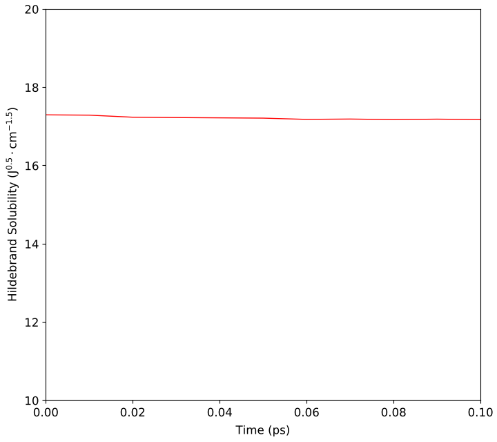
Fig. 146 Calculated Hildebrand solubility of PVC.

Notes

This class enables the calculation of the cohesive energy density of a polymer system from either a MDTrajectory or BulkConfiguration.

The cohesive energy of a polymer system is the energy required to completely separate all of the polymer chains from each other. It therefore consists of the non-bonding interactions between polymer chains, and gives a measure of their attractiveness to each other. In bulk systems this energy is normally expressed per unit of volume of the material, giving the cohesive energy density. The relative differences in cohesive energy densities of different polymers indicates their miscibility or immiscibility with each other. One important measure of the solubility of a polymer is the Hildebrand solubility parameter, \(\delta_h\). This is simply given as:

\[\delta_h = \sqrt{\frac{E_{coh}}{V}}\]

Here \(E_{coh}\)is the cohesive energy density of the unit cell and \(V\) is the cell volume. Polymers with a difference in solubility of less than 2MPa^0.5 are generally expected to be miscible[1].

A more precise measure of miscibility is given through the Flory-Huggins parameter \(\chi\)[2]. For a binary mixture composed of polymers \(A\) and \(B\), the volume fraction of each polymer \(\phi\) can be given as:

\[\phi_A = \frac{n_A r_A}{n_A r_A + n_B r_B}\]

Here \(n\) is the number of polymer chains and \(r\) is the number of monomers per polymer chain. Given the volume fraction of each polymer, the free energy of mixing \(\Delta G\) can be approximated as:

\[\Delta G = RT\left(\frac{\phi_A}{r_A}\ln \phi_A + \frac{\phi_B}{r_B}\ln \phi_B + + \phi_A \phi_B \chi_{AB} \right)\]

Here \(\chi_{AB}\) is the Flory-Huggins parameter for the polymer mixture. In this equation the first two terms specify the entropy of mixing, while the last term approximates the enthalpy of mixing. The Flory-Huggins parameter is therefore a measure of the enthalpy of mixing.

Using a mean-field approximation the Flory-Huggins parameter can be given as:

\[\chi_{AB} = \frac{V_{mono}}{RT}\left[\phi_A \left(\frac{E_{coh}}{V}\right)_A + \phi_B \left(\frac{E_{coh}}{V}\right)_B - \left(\frac{E_{coh}}{V}\right)_{mix} \right]\]

Here \(V_{mono}\) is the average volume per monomer. In this approximation it is assumed that both monomers have similar sizes, and so size difference does not need to be taken into account when calculating thermodynamics of mixing. This definition also assumes that the two systems are in contact both with themselves and each other. This is not the case in dilute solutions where one polymer chain may be completely surrounded by others. To calculate the Flory-Huggins parameter the cohesive energy densities of both the pure polymers and the polymer blend is required. In this way, specific interactions between polymers, such as hydrogen bonding, is taken into account in the estimation of miscibility. It should also be noted that, unlike the Hildebrand solubility, the Flory-Huggins parameter is also explicitly a function of temperature. Temperature changes in the system can also indirectly alter the amount of cohesive energy in the system, as thermal motions push the configuration away from equilibrium. Polymer blends with a Flory-Huggins parameter below the critical value are expected to be miscible[1]. The critical Flory-Huggins value \(\chi_c\) can be given as:

\[\chi_c = \frac{1}{2}\left(\frac{1}{\sqrt{r_A}} + \frac{1}{\sqrt{r_B}}\right)^2\]

To calculate the cohesive energy density of a polymer system a CohesiveEnergyDensity object first needs to be created. This takes a MDTrajectory or BulkConfiguration representing the polymer system. The specific images in the MDTrajectory to analyzed can be selected using the start_time, end_time and time_resolution arguments. The polymer chains analyzed in the configuration can be specified with the polymer_tags argument. This takes a list of tags of polymer molecules in the configuration. By default polymers tagged with POLYMER_MOLECULE_# are analyzed, where # is a numerical index. The flag Automatic can also be used to automatically identify polymer chains using the bond graph in the configuration.

To calculate the interaction energy of the polymers, the existing forcefield calculator on the trajectory is used. The accuracy of this calculator can be modified with some additional arguments. The argument nonbond_cutoff controls the cutoff used to evaluate the non-bonding Lennard-Jones potentials. Likewise it is possible to change the electrostatic summation method. By default the summation method defined in the calculator is used. If no electrostatic summation method is set and no electrostatic summation arguments are given, then electrostatic interactions are not included in the calculation of cohesive energy. SPME summation can be used by setting the accuracy of this summation with the argument electrostatic_accuracy. Damped shifted-force electrostatic summation can also be used by setting the argument use_coulomb_dsf to True and giving a cutoff using the electrostatic_cutoff argument. By default the same methods in the attached calculator are used to calculate the cohesive energy. This is also generally the most appropriate use as this is the potential that was used to construct the system.

In addition to the cohesive energy density of the whole system, it is also possible to calculate the interaction energy of each individual polymer chain with the remainder of the system. This is specified by setting the argument calculate_interaction to True. Finally it is possible to set whether the MDTrajectory used to calculate the cohesive energy is cached in memory or read from disk during the calculation. Caching in memory is faster, but for very large trajectories may exhaust available memory. By default trajectories are cached in memory. To force reading from disk, set the argument memory_cache to False.

Once the object is created the properties of the polymer system can be returned using query methods. The unit cell volumes of each selected image can be returned with the volumes methods. The cohesive energy and cohesive energy density can be returned with the methods cohesiveEnergies and cohesiveEnergyDensities respectively. The Hildebrand solubility can be returned with the method solubilities. The method totalEnergies returns the total non-bonding energy of each image. The method nonMolecularEnergies returns the internal non-bonding energy of the atoms in each image that are not associated with a polymer tag. For example, in the case where the system contains a metal surface, nonMolecularEnergies returns the internal non-bonding energy of that surface. Finally the methods moleculeEnergies and interactionEnergies return the internal non-bonding energy and the interaction energy of each polymer molecule respectively. In these methods the polymer molecules are indexed using their tags. The method interactionEnergies is also only available if the calculation of interaction energies was specified when the CohesiveEnergyDensity object was created by setting the argument calculate_interaction to True.

[1] (1,2)

Zhonglin Luo and Jianwen Jiang. Molecular dynamics and dissipative particle dynamics simulations for the miscibility of poly(ethylene oxide)/poly(vinyl chloride) blends. Polymer, 51:291, 2010. URL: https://www.sciencedirect.com/science/article/abs/pii/S0032386109010040, doi:10.1016/j.polymer.2009.11.024.

[2]

Paul J. Flory. Statistical thermodynamics of polymer solutions, pages 495–540. Cornell University Press, 1953.