CollectiveVariableHyperdynamics
Included in QATK.Dynamics
- class CollectiveVariableHyperdynamics(distortions, temperature=None, global_exponent=None, global_cut=None, gaussian_width=None, gaussian_height=None, gaussian_frequency=None, bias_damping_temperature=None, gaussian_limit=None, reaction_steps=None, optimize_new_state=None, measurement_frequency=None, tracked_atoms_tag=None, allow_no_variables=None)
Hook function implementing collective variable hyperdynamics.
- Parameters:
distortions (Sequence of
HyperdynamicsBaseDistortion) – The geometric distortions used to create the collective variable.temperature (PhysicalQuantity of type temperature |
None) – The temperature of the simulation, used for calculating the hypertime. Default: 300 Kelvinglobal_exponent (float) – The exponent used to create the global distortion. Default: 6
global_cut – The value of the global distortion at the transition state. This can be used to set the position of the transition state where individual distortions do not range from 0 to 1. One example of this is when using a bond distortion without a maximum bond length. Default: 1
gaussian_width (float) – The width of the added Gaussian bias potential. Default: 0.025
gaussian_height (PhysicalQuantity of type energy) – The height of the added Gaussian bias potential. Default: 0.01 eV
gaussian_frequency (int) – The number of steps between adding new Gaussian bias potentials. Default: 1000
bias_damping_temperature (PhysicalQuantity of type temperature |
None) – The temperature used to scale the bias potential using well-temperated metadynamics.Nonedoes not damp the added potential, resulting the in same size potential being added at each step. Default:Nonegaussian_limit (float) – The upper limit in the collective variable where Gaussians are added to the hyperdynamic bias potential. Gaussians are not added at values above this limit in order to avoid biasing the transition state. Default: 1.0
reaction_steps (int) – The number of steps at the maximum collective variable before a reaction takes place. Default: 5000
optimize_new_state (bool) – Use an optimized configuration to reset the distortions after a reaction is detected. Default: True
measurement_frequency (int) – The step frequency with which measurements are added to the trajectory. Default: 10
tracked_atoms_tag (str) – Tag giving the indices of atoms for which the position is measured during the simulation.
Noneresults in no atoms being tracked. Default:Noneallow_no_variables (bool) – Continue in cases where no variables are found for acceleration. The simulation continues the number of reaction steps without bias before trying again to find variables to accelerate. Default: True
- allowNoVariables()
- Returns:
True if the simulation continues in cases where no variables are found for acceleration.
- Return type:
bool
- biasDampingTemperature()
- Returns:
The temperature used to scale the bias potential.
- Return type:
PhysicalQuantity of type temperature
- callInterval()
- Returns:
The call interval of this hook function.
- Return type:
int
- distortions()
- Returns:
The geometric distortions used to create the collective variable.
- Return type:
Sequence of
HyperdynamicsBaseDistortion
- gaussianCenters()
- Returns:
The center of the Gaussian potentials added to form the bias potential.
- Return type:
ndarray
- gaussianFrequency()
- Returns:
The frequency at which new Gaussian bias potentials are added.
- Return type:
int
- gaussianHeight()
- Returns:
The height of the Gaussian bias potential.
- Return type:
PhysicalQuantity of type energy
- gaussianHeights()
- Returns:
The height of the Gaussian potentials added to form the bias potential.
- Return type:
PhysicalQuantity of type energy
- gaussianLimit()
- Returns:
The limit in the collective variable above which Gaussians are not added.
- Return type:
float
- gaussianWidth()
- Returns:
The width of the Gaussian bias potential.
- Return type:
float
- gaussianWidths()
- Returns:
The widths of the Gaussian potentials added to form the bias potential.
- Return type:
ndarray
- globalCut()
- Returns:
The value of the global distortion at the transition state.
- Return type:
float
- globalExponent()
- Returns:
The global exponent used in the collective variable.
- Return type:
float
- measurementFrequency()
- Returns:
The step frequency with which measurements are saved to the trajectory.
- Return type:
int
- numberOfGaussians()
- Returns:
The number of Gaussian potentials added to form the hyperdynamic bias potential.
- Return type:
int |
None
- numberOfVariables()
- Returns:
The total number of geometric coordinates being accelerated. If the geometric coordinates are not set with a configuration
Noneis returned.- Return type:
int |
None
- optimizeNewState()
- Returns:
True if the configuration is optimized before setting new distortions.
- Return type:
bool
- reactionSteps()
- Returns:
The number of steps at the maximum collective variable before a reaction takes place.
- Return type:
int
- temperature()
- Returns:
The simulation temperature.
- Return type:
PhysicalQuantity of type temperature
- trackedAtomsTag()
- Returns:
The tag for the atoms that are tracked during the simulation.
- Return type:
str
- uniqueString()
Return a unique string representing the state of the object.
Usage Examples
In this example collective variable hyperdynamics is used to study the diffusion of a single hydrogen atom in a copper crystal lattice. A position distortion is used to add a bias potential to push the atom through the lattice. The results of the simulation are recorded in the resulting MDTrajectory and can be viewed in the Movie Tool. The resulting diffusivity can also be calculated using the IrregularTimeMeanSquareDisplacement object.
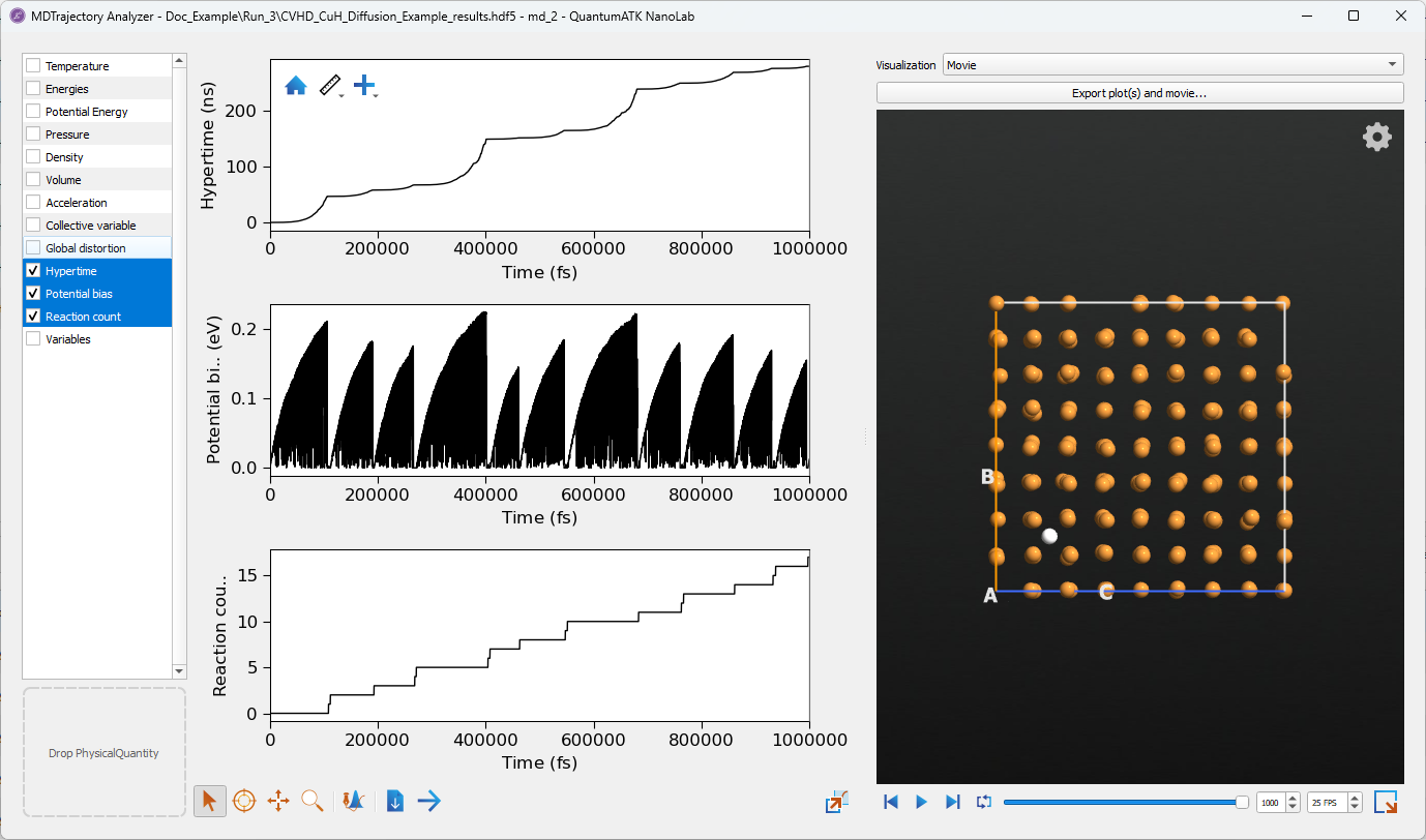
This simulation may take several hours to run. Note that the simulation performs a limited amount of sampling, using
only a million steps or 1ns of simulation time. The hypertime of the simulation however is over 250ns, meaning that the
simulation was able to effectively sample this time for the cost of only 1ns of simulation. At 300 Kelvin the diffusion
of hydrogen in copper is around \(8.5 \times 10^{-14} m^2/s\) so very long trajectories are needed to measure the
slow diffusion[1]. For accurate results it is necessary to use either more steps or to run
multiple simulations. Running multiple simulations can enable a faster turn-around time, as the simulations can be run
parametrically in parallel. The workflow for this example can be
downloaded here with the corresponding Python script
CVHD_CuH_Diffusion_Example.py.
Notes
Hyperdynamics is a method for sampling rare events using molecular dynamics. In hyperdynamics a bias potential is added to degrees of freedom separating different states. The bias potential aids in lowering the energy barrier between these states, allowing the system to sample different states more freely. In this way the biased degrees of freedom move at elevated temperature, while the rest of the system moves at the simulation temperature. The acceleration factor given to the system by the bias potential can be calculated as the ensemble average of the bias potential. When this boost factor is multiplied by the simulation time it gives the effective sampling time, known as the hypertime.
In using the hypertime to estimate reaction rates, it is important that the bias potential is not applied at the transition state. If bias is applied both at the reactant and transition state it obscures the relative free energy barrier between two states. This can lead to errors in estimations of the rate constant. This also applies to kinetic based processes such as diffusion.
In collective variable hyperdynamics the bias potential is built up during the simulation by adding Gaussian functions to the potential at the value of the collective variable during the simulation[2]. By building up the potential it avoids requiring knowledge of the the appropriate shape or height of the bias potential. This is distinct from StaticHyperdynamics, which requires some knowledge of the transition state barrier height. In this way collective variable hyperdynamics is similar to metadynamics. The main difference is that in metadynamics a single bias potential is built up during the simulation. This is converged to create an estimate of the total free energy of a process in the system. In hyperdynamics the bias potential is simply used to accelerate a defined reaction. Once the reaction occurs, the bias potential is reset to zero and is built up again at the new reactant. Rather than the free energy profile, the important results from hyperdynamics simulations are the trajectory and the effective hypertime of the simulation.
In order to create the bias potential, one or more important geometric features, known as distortions, are first identified in the configuration. These can be things such as the position of atoms or the bond lengths between specific atoms. These distortions are generally constructed so that they range from 0 to 1 when moving from reactant to transition state. The different distortions are then combined into a global distortion through the equation:
Here \(\chi_t\) is the global distortion and \(\chi_i\) are the individual distortions. The power \(p\)
increases the contribution of the larger distortions to the global distortion. In the
CollectiveVariableHyperdynamics class the distortions are given as a list using the distortions argument.
These can be either HyperdynamicsPositionDistortion objects or HyperdynamicsBondDistortion
objects. The exponent \(p\) is set using the global_exponent keyword argument.
To ensure that the gradients at the boundaries are zero, the collective variable is then defined using a cosine function such that:
Here \(\eta\) is the collective variable and \(\chi_c\) is a cutoff value of the global distortion. This is
the value of the global distortion at the transition state. In the simplest case in which one distortion that ranges
from 0 to 1 is used, this is simply one. If a combination of distortions are used, or if the distortions do not
range from 0 to 1 the \(\chi_c\) is used to make the collective variable range from 0 to 1. This cutoff value is
set using the global_cut keyword argument. The collective variable is also used to determine when a reaction has
occurred in the configuration. When the collective variable is greater than 1 for a set number of steps the system is
considered to have reacted, and the references for distortions and the bias potential is reset to zero. The number of
steps used to determine if a reaction has occurred is set with the reaction_steps keyword argument. By default this
is set to 5000 steps. In setting the new distortions the reference configuration can first be optimized using
the current calculator. This ensures that the distortions are set from a local energy minimum. In the case of bonds it
ensures that the correct bonds are selected for boosting. Likewise in the case of positions that the reference positions
are at a potential minimum. This optimized reference configuration is not used in the dynamics simulation, as to do so
would alter the sampling of different states. It is in general recommended to optimize the reference configuration.
Enabling optimization after reactions is done with the optimize_new_state keyword argument, which is
True by default.
After each reaction the distortion definitions are reset to the new reference configuration. In some cases, such as
bonds being boosted, it means that a different number of distortions may be selected. This can also include cases
where no available distortions are found that can be accelerated. In this case the simulation can simply continue
the number of steps between reactions and try again to find some applicable distortions. Alternatively the simulation
can simply end if no distortions indicates that something has gone wrong with the simulation. Stopping on no distortions
being found is controlled with the allow_no_variables keyword argument. By default this is set to True,
meaning that the simulation will continue.
The total bias potential \(\Delta V(\eta)\) is calculated by adding Gaussians at time intervals \(\tau_G\). This gives the expression for the total bias potential:
Here \(w_k\) is the height of the Gaussian and \(\delta\) is the Gaussian width. These can be set with the
keyword arguments gaussian_height and gaussian_width respectively. The number of steps between adding Gaussians
is also set with the gaussian_frequency keyword argument. Together with the Gaussian height and width this sets the
rate of energy deposition into the bias during the simulation. The optimal energy deposition rate depends on the depth
of the local potential well and the temperature of the simulation. The energy deposition rate should be low enough to
allow for effective sampling of the reactant potential energy surface so that a reliable estimate of the hypertime is
obtained.
The height of each added Gaussian can also be scaled down depending on the amount of bias already added at the
collective variable.This is similar to the well-tempered metadynamics method, where the bias potential converges to a
value based on a temperature used to set the rate of reducing the size of the added Gaussians. Using this method the
temperature is proportional to the maximum effective temperature of the motion of the collective variable. Reducing
the temperature reduces the energy deposition rate into the bias potential. The temperature used to set the height of
the Gaussians is given with the bias_damping_temperature keyword argument. Here None means that no damping is
done and that all added Gaussians have the same height. In order to avoid adding bias at the transition state,
Gaussians can be added up to a limit in the collective variable. This limit depends on the width of the Gaussians and
how close to the true transition state the collective variable extends to. This limit is set with the
gaussian_limit keyword argument.
For each reaction the hypertime is calculated as the simulation time multiplied by the ensemble average of the bias potential. This is given as:
Here \(t_h\) is the hypertime, \(t_s\) is the simulation time and \(T\) is the simulation temperature. This
is set with the temperature keyword argument. Note that as the bias potential is built up over the simulation,
it is dependent on the time. When a new reaction is found the bias potential starts off as zero. At this point both
the simulation time and hypertime move at the same rate. As the bias potential is built up the hypertime moves
increasingly faster until a new reaction is found and the bias potential is reset. To get an accurate measure of the
hypertime it is important to have sufficient sampling of areas of high bias. This can limit the bias energy deposition
rate. If is is too high sufficient sampling of the bias potential may not occur.
When running a collective variable hyperdynamics simulation in MolecularDynamics, information about the
simulation, such as the hypertime, current bias potential and collective variable value are added to the trajectory
as measurements. These are shown in the Movie Tool when opening the trajectory. The number of steps between adding
measurements is set using the measurement_frequency keyword argument. Additionally the positions of select
atoms can be added as a measurement. This is useful in cases where the diffusion of single atom impurities
is being studied. These are added with the measurement name tracked_atoms. As this is an array of atomic
coordinates it cannot be displayed in the Movie Tool. The tag of the atoms to track is given with the
tracked_atoms_tag keyword argument. If no tag is given atom tracking is not added to the trajectory.
To calculate diffusion from a hyperdynamics simulation the IrregularTimeMeanSquareDisplacement class can be used. This class can access both the hypertime and tracked atomic positions from the trajectory and calculated the resulting mean square displacement of the tracked atoms. As diffusion is a stochastic process, it is often useful to run several simulations to fully sample the motion of the atoms. This is especially true for amorphous systems or systems lacking long-range order.