DeviceDensityOfStates
Included in QATK.Analysis
- class DeviceDensityOfStates(configuration, energies=None, kpoints=None, contributions=None, self_energy_calculator=None, energy_zero_parameter=None, infinitesimal=None)
Constructor for the Device Density of States object.
- Parameters:
configuration (
DeviceConfiguration) – The one or two-probe configuration with attached calculator for which the density of states. should be calculated.energies (PhysicalQuantity of type energy.) – The energies for which the density of states should be calculated. Default:
numpy.linspace(-2., 2., 200)*eVkpoints (sequence (size 3) of int |
MonkhorstPackGrid|KpointDensity|RegularKpointGrid) – The k-points for which the density of states should be calculated. Note that the k-points must be in the xy-plane. Default:MonkhorstPackGrid(na, nb)where(na, nb)is the sampling used for the self-consistent calculation.contributions (
Left|Right|All) – The density contributions to include in the density of states. Default:Allself_energy_calculator (
RecursionSelfEnergy|SparseRecursionSelfEnergy) – The self energy calculator to be used for the density of states. Default:RecursionSelfEnergy(storage_strategy=NoStorage())energy_zero_parameter (
AverageFermiLevel|AbsoluteEnergy.) – Specifies the choice for the energy zero. Default:AverageFermiLevelinfinitesimal (PhysicalQuantity of type energy.) – Small energy, used to move the density of states calculation away from the real axis. This is only relevant for recursion-style self-energy calculators. Default:
1.0e-6*eV
- bias()
- Returns:
The applied bias.
- Return type:
PhysicalQuantity type voltage.
- electrodeFermiLevels()
- Returns:
The Fermi levels of the left and right electrodes in absolute energies.
- Return type:
PhysicalQuantity of type energy.
- electrodeFermiTemperatures()
- Returns:
The Fermi temperature of the left and right electrodes used in this density of states.
- Return type:
PhysicalQuantity of type temperature.
- electrodeVoltages()
- Returns:
The left and right electrode_voltages used in this density of states spectrum.
- Return type:
PhysicalQuantity of type voltage.
- elements()
- Returns:
The elements in the configuration used for generating the density of states.
- Return type:
list of
PeriodicTableElement
- energies()
- Returns:
The energies used in this density of states.
- Return type:
PhysicalQuantity of type energy.
- energyZero()
- Returns:
The energy zero used for the energy scale in this density of states.
- Return type:
PhysicalQuantity of type energy.
- evaluate(spin=None, projection_list=None)
Evaluate the density of states.
- Parameters:
spin (
Spin) – The spin component. Default:Spin.Sumprojection_list (
ProjectionList) – ProjectionList with projections to include in the density of states. Default:ProjectionList(range(n_left, n_central-n_right))
- Returns:
The density of states for the given spin component. For the spin Spin.All, a list containing the density of states for Spin.Sum, Spin.X, Spin.Y and Spin.Z is returned.
- Return type:
PhysicalQuantity | list(4) of PhysicalQuantity
- infinitesimal()
- Returns:
The infinitesimal used for calculating the density of states.
- Return type:
PhysicalQuantity of type energy.
- metatext()
- Returns:
The metatext of the object or None if no metatext is present.
- Return type:
str | None
- nlinfo()
Returns information about the DeviceDensityOfStates object.
- Returns:
A dictionary containing the DeviceDensityOfStates information.
- Return type:
dict
- nlprint(stream=None)
Print a string containing an ASCII table useful for plotting the AnalysisSpin object.
- Parameters:
stream (python stream) – The stream the table should be written to. Default:
NLPrintLogger()
- numberOfElectrodeAtoms()
- Returns:
The number of atoms in each electrode in the configuration used for generating the density of states.
- Return type:
tuple of int.
- setMetatext(metatext)
Set a given metatext string on the object.
- Parameters:
metatext (str | None) – The metatext string to set. Use “None” to remove current metatext.
- spins()
- Returns:
The spins used in this density of states.
- Return type:
tuple of spin component flags.
- uniqueString()
Return a unique string representing the state of the object.
Usage Examples
Calculate the DeviceDensityOfStates (DDOS) of a Li-H2-Li system:
# setup Huckel calculation for Li-H2-Li device

electrode_lattice = UnitCell([8., 0., 0.]*Angstrom,
                             [0., 8., 0.]*Angstrom,
                             [0., 0., 8.7]*Angstrom)

electrode_elements = [Lithium, Lithium, Lithium]
electrode_coordinates = [ [ 4.,  4., 1.45+i*2.9] for i in range(3)]*Angstrom

electrode = BulkConfiguration(
    bravais_lattice=electrode_lattice,
    elements=electrode_elements,
    cartesian_coordinates=electrode_coordinates
    )

lattice = UnitCell([8., 0., 0.]*Angstrom,
                   [0., 8., 0.]*Angstrom,
                   [0., 0., 37.376]*Angstrom)

elements = [Lithium,]*6 +[Hydrogen,]*2+[Lithium,]*6

coordinates = [ [ 4.,  4., 1.45+i*2.9] for i in range(6)] + \
              [ [ 4.,  4., 18.286+i*0.8] for i in range(2)] + \
              [ [ 4.,  4., 21.426+i*2.9] for i in range(6)]

central_region = BulkConfiguration(
    bravais_lattice=lattice,
    elements=elements,
    cartesian_coordinates=coordinates*Angstrom
    )

device_configuration = DeviceConfiguration(
    central_region,
    [electrode, electrode]
    )

calculator = DeviceHuckelCalculator(
    iteration_control_parameters = NonSelfconsistent,
    )

device_configuration.setCalculator(calculator)

device_configuration.update()
nlsave('device.nc', device_configuration)

#setup energies, and calculate DOS
energies = numpy.linspace(-2,3,100) * eV
dos = DeviceDensityOfStates(device_configuration, energies=energies)
nlsave('device.nc', dos)
Plot the projected density of states (PDOS) for the non-surface atoms of the central region:
# read the dos
dos = nlread('device.nc',DeviceDensityOfStates)[0]
conf = nlread('device.nc', DeviceConfiguration)[0]
energies = dos.energies()

# calculate projection on atoms in the central region
dos_projection = [dos.evaluate(projection_list = ProjectionList([i])) \
                  for i in range(3,11)]

# plot the projections
import pylab
pylab.figure()
for i in range(3,11):
    label = conf.elements()[i].symbol()+'('+str(i)+')'
    pylab.plot(energies.inUnitsOf(eV),dos_projection[i-3].inUnitsOf(eV**-1), \
               label = label)
pylab.legend()
pylab.xlabel("Energy (eV)")
pylab.ylabel("dos (1/eV)")
pylab.show()
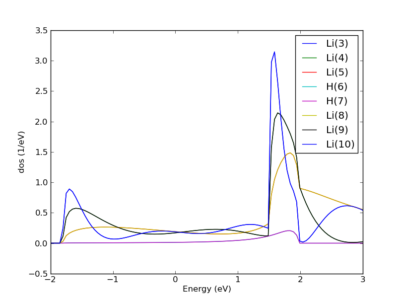
Fig. 170 The density of states of the Li-H2-Li systems projected onto the atoms in the central region. Note that half of the curves are not visible because they fall on top of the other curves due to symmetry.
Calculate the contribution to the density of states from scattering states originating in the left electrode:
conf = nlread('device.nc',DeviceConfiguration)[0]

#setup energies
energies = numpy.linspace(-2,3,100) * eV

#calculate the dos from the Left electrode
dos = DeviceDensityOfStates(conf, energies=energies, contributions=Left)

#calculate the projections on the atoms in the central region
dos_projection = [
     dos.evaluate(projection_list = ProjectionList([i])) for i in range(3,11)
     ]

#plot the data
import pylab
pylab.figure()
for i in range(3,11):
    label = conf.elements()[i].symbol()+'('+str(i)+')'
    pylab.plot(
        energies.inUnitsOf(eV),
	dos_projection[i-3].inUnitsOf(eV**-1),
	label=label
	)
pylab.legend()
pylab.xlabel("Energy (eV)")
pylab.ylabel("dos (1/eV)")
pylab.show()
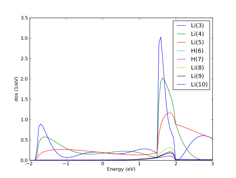
Fig. 171 The density of states from the left electrode of the Li-H2-Li systems projected onto the atoms in the central region. Note how the density of states in the right lithium atoms is reduced due do damping of the propagation by the hydrogen molecule.
Do the k-point average of the DOS:
dos = DeviceDensityOfStates(conf,
                            kpoints=MonkhorstPackGrid(4,4),
                            energies=energies,
                            contributions=Left)
Notes
The routine utilizes the symmetries of the configuration to reduce the computational load for k-point averaging.
The DeviceDensityOfStates (DDOS) \(D(E)\) is computed via the spectral density matrix \(\rho(E)=\rho^L(E)+\rho^R(E)\) (cf. The non-equilibrium Green’s function (NEGF) method) where \(L/R\) denotes the contribution from the left/right electrode (see the keyword contributions above).
The local density of states (LDOS) is defined as
where we note that the basis set orbitals \(\phi_i(\mathbf{r})\) are real functions in QuantumATK through the use of solid harmonics.
The device density of states is then obtained by integrating the LDOS over all space:
where \(S_{ij}=\int \phi_i(\mathbf{r})\phi_j(\mathbf{r})d\mathbf{r}\) is the overlap matrix. Introducing \(M_{i}(E)=\sum_j \rho_{ij}(E) S_{ij}\), we may write this as
where thus \(M_i(E)\) can be seen as the contribution to the DDOS from orbital \(i\). \(M_i(E)\) is a spectral MullikenPopulation, with
\(M_i(E)\) can be summed over orbitals of a particular angular momentum and/or over one or several atoms to give the projected device density of states (PDDOS). This can also be plotted in QuantumATK. The projection is specified via the projection_list keyword to the evaluate() method (see above).