FiniteBiasSpinTransferTorque

class FiniteBiasSpinTransferTorque(configuration, filename, object_id, atom_indices=None, bias_voltages=None, kpoints=None, initial_spin=None, potential_drop_region_tags=None, potential_drop_method=None, potential_profile=None, number_of_processes_per_task=None, log_filename_prefix=None, initial_state=None)

configuration:

The device calculation that the finite bias spin transfer torque should be calculated for.

configuration:

DeviceConfiguration

Parameters:

• filename (str) – The full or relative filename path the study object should be saved to. See nlsave().

• object_id (str) – The name of the study that the study object should be saved to within the file. This needs to be a unique name in this file.

• atom_indices (list of int | list of str) – The indices of the atomic sites to calculate the spin transfer torque for. This may be defined as a list of integers or a list of tags.
  Default: All atoms in the configuration

• bias_voltages (PhysicalQuantity of type voltage) – A list of voltages. Each voltage will in turn represent the value 1.0 in the potential profile when converting the latter to the voltage drop profile accross the device. I.e. if the potential profile drops by 1.0 from the left to the right lead the voltage drop from the left to the right lead will equal each given voltage in turn.
  Default: numpy.linspace(-0.5, 0.5, 11)*Volt

• kpoints (MonkhorstPackGrid | KpointDensity) – The k-points for which the spin transfer torque should be calculated.
  Default: The Monkhorst-Pack grid used for the self-consistent calculation.

• initial_spin (InitialSpin) – The initial spins of the device for the non-collinear calculation.
  Default: Initial spin where all spins are pointing in the x-direction (theta=90, phi=0) except for the atoms in atom_indices, which will be pointing in the z-direction (theta=0, phi=0)

• potential_drop_region_tags (list of str) – List of tags defining regions where the potential drops. A potential profile will be generated automatically based on the tagged regions. It is a requirement that the tagged regions do not overlap in the z-direction.
  Default: None

• potential_drop_method (str) – Parameter describing how the potential drops as function of length. This should either be ‘linear’ or ‘exponential’
  Default: ‘exponential’

• potential_profile (List of (PhysicalQuantity of type length, float)) –

  Defines the potential model as a piecewise linear function, defined as a list of (coordinate, value) pairs, where the values define the potential drop in an interval \((+V_b/2, V_b/2)\) with \(V_b\) the applied bias.

  For example, a list [(0*Ang, 1), (5*Ang, 1), (10*Ang, 0.), (15*Ang, 0.), (20*Ang, -1.), (25*Ang, -1.)] represents a potential ramp from \(V_b/2\) to \(-V_b/2\) between coordinates 5 and 20 Angstrom, with a flat 0 potential region in the middle. It is required that the leftmost and rightmost values are 1 and -1 respectively.

  If potential_profile this will be used for the non-self consistent potential drop.
  Default: [(0*Ang, 1), (L_C, -1)], where L_C is the central region length.

• number_of_processes_per_task (int | None | ProcessesPerNode) – The number of processes that will be used to execute each task. If the total number of processes does not divide evenly into the tasks, some tasks may have less than this number of processes. If None, all available processes execute each task collaboratively.
  Default: None

• log_filename_prefix (str | LogToStdOut) – Filename prefix for the logging output of study object. If LogToStdOut, all logging will instead be sent to standard output.
  Default: 'srhrecombination_'

atomIndices()

Returns:

The indices of the atomic sites to calculate the spin transfer torque for.

Return type:

list of int

atomResolvedSpinTransferTorkance(atom_indices=None)

Returns:

Linear response spin transfer torkance array of shape (3, n_atom_indices), where the 3 corresponds to x, y, z directions.

Return type:

PhysicalQuantity of type energy per voltage (charge).

atomResolvedSpinTransferTorques(atom_indices=None, bias_voltages=None)

Parameters:

• atom_indices (list of int | All) – List of atom indices to sum the STT contribution over. If All or None, the indices used at construction will be used.

• bias_voltages (PhysicalQuantity of type voltage) – A list of voltages for which to get the result.
  Default: All the bias voltages used at construction.

Returns:

Spin transfer torque array of shape (n_bias_points, 3, n_atom_indices), where the 3 corresponds to x, y, z directions.

Return type:

PhysicalQuantity of type energy

biasVoltages()

Returns:

The bias voltages.

Return type:

PhysicalQuantity of type Volt

calculator()

Returns:

The calculator attached to the configuration.

Return type:

DeviceLCAOCalculator

dependentStudies()

Returns:

The list of dependent studies.

Return type:

list of Study

filename()

Returns:

The filename where the study object is stored.

Return type:

str

initialSpin()

Returns:

The initial spin to be used for the non-collinear calculation.

Return type:

InitialSpin

kpointResolvedSpinTransferTorkance(atom_indices=None)

Parameters:

atom_indices (list of int | All) – List of atom indices to sum the STT contribution over. If All or None, the indices used at construction will be used.

Returns:

Spin transfer torkance array of shape (3, n_kpoints), where the 3 corresponds to x, y, z directions. The torkance is summed over atom indices.

Return type:

PhysicalQuantity of type energy per voltage (charge).

kpointResolvedSpinTransferTorques(bias, atom_indices=None)

Parameters:

• bias (PhysicalQuantity of type Volt) – The bias voltage to get result from.

• atom_indices (list of int | All) – List of atom indices to sum the STT contribution over. If All or None, the indices used at construction will be used.

Returns:

Spin transfer torque array of shape (3, n_kpoints), where the 3 corresponds to x, y, z directions. The STT is summed over atom indices.

Return type:

PhysicalQuantity of type energy

kpoints()

Returns:

The k-points for which the spin transfer torque is calculated.

Return type:

MonkhorstPackGrid

logFilenamePrefix()

Returns:

The filename prefix for the logging output of the study.

Return type:

str | LogToStdOut

nlprint(stream=None)

Print a string containing an ASCII table useful for plotting the Study object.

Parameters:

stream (python stream) – The stream the table should be written to.
Default: NLPrintLogger()

numberOfProcessesPerTask()

Returns:

The number of processes to be used to execute each task. If None, all available processes execute each task collaboratively.

Return type:

int | None | ProcessesPerNode

numberOfProcessesPerTaskResolved()

Returns:

The number of processes to be used to execute each task. Default values are resolved based on the current execution settings.

Return type:

int

objectId()

Returns:

The name of the study object in the file.

Return type:

str

potentialProfile()

Returns:

Defines the potential model as a piecewise linear function, defined as a list of (coordinate, value) pairs.

Return type:

List of (PhysicalQuantity of type length, float)

potentialProfileCoordinates()

Returns:

The coordinates in the potential profile model.

Return type:

list of PhysicalQuantity of type length

potentialProfileValues()

Returns:

The scaling values in the potential profile model.

Return type:

list of float

saveToFileAfterUpdate()

Returns:

Whether the study is automatically saved after it is updated.

Return type:

bool

totalSpinTransferTorkance()

Returns:

Spin transfer torque array of shape (n_bias_points, 3), where the 3 corresponds to x, y, z directions.

Return type:

PhysicalQuantity of type energy per voltage (charge).

totalSpinTransferTorques()

Returns:

Spin transfer torque array of shape (n_bias_points, 3), where the 3 corresponds to x, y, z directions.

Return type:

PhysicalQuantity of type energy

uniqueString()

Return a unique string representing the state of the object.

update()

Run the calculations for the study object.

Usage Examples

In this example we will calculate the spin transfer torque (STT) in a Fe-MgO-Fe magnetic tunneling junction (MTJ) as shown below. The left Fe, MgO, and right Fe regions have been assigned the tags ‘layer 0’, ‘layer 1’, and ‘layer 2’ respectively. We will be calculating the STT in free layer, which we will define as layer 2, for an angle of 90 degree between the magnetization in the left (layer 0) and free (layer 2) magnetic regions.

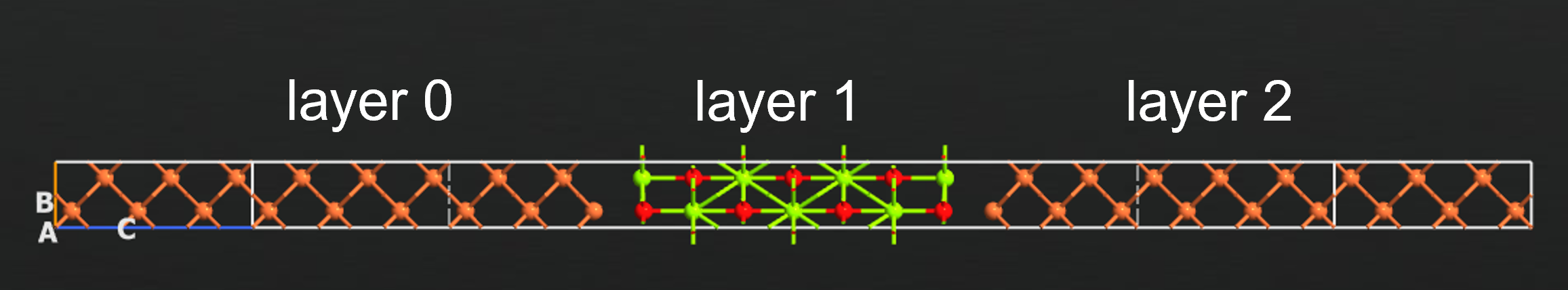
The spin transfer torque is evaluated in a non-selfconsistent finite bias approximation. The potential drop across the MgO barrier is represented as a linear ramp across the tunneling barrier [1], avoiding time consuming and often hard to converge non-collinear calculations at finite bias. The specification of the potential drop region is most easily done using tags.

The figure below shows how to setup the calculation using the work flow builder and the FiniteBiasSpinTransferTorque editor.

The free layer atoms, where the STT will be evaluated can be specified in the editor using tags, setting it to ‘layer 2’ in this example. The potential drop region is likewise specified using tags, in this case ‘layer 1’.

A workflow for the calculation can be downloaded here with a corresponding python script Fe-MgO-Fe-STT-Medium.py. Note that the DeviceLCAOCalculator needs to have spin set to Noncollinear.

Note

The calculation will take several hours, even when running on multiple cores.

Initial spin

When setup like above, the STT will be calculated for a spin configuration defined as

• The spin in the free layer (layer 2) is oriented along the z-axis

• The spin in the left Fe layer (layer 0) is rotated with \(\theta=90^\circ\) and \(\phi=0^\circ\) pointing in the x-direction.

• The spin in the potential drop region is scaled to zero.

This means that the in-plane component of the STT vector will be in the x-direction, while the out-of-plane component will be in the y-direction.

It is possible to define a custom spin orientation, by inserting an InitialSpin block before the FiniteBiasSpinTransferTorque work-flow block.

Analyze results

When the calculation has finished the results can be visualized with the Finite bias spin transfer torque analyzer as illustrated below.

The total STT on the free layer atoms

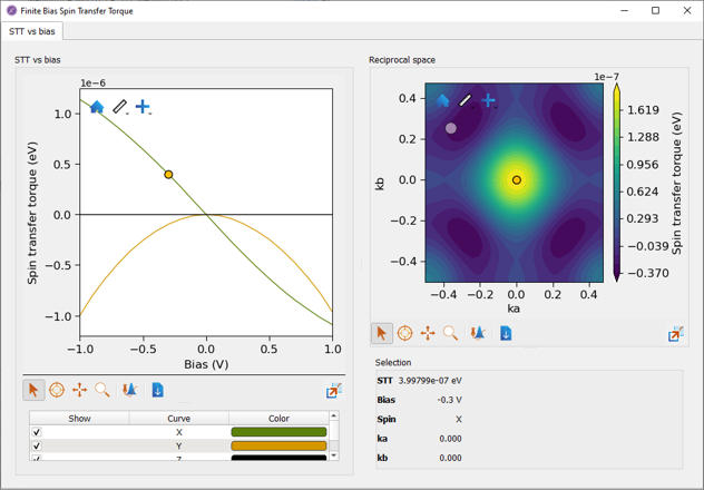
The close to linear behavior of the in-plane (x-) component for small bias and the quadratic behavior of the out-of-plane (y-) component are consistent with literature results [2], [1].

Note

Results can be sensitive to numerical parameters such as k-point sampling or real axis contour accuracy. Convergence with respect to those parameters should be carefully checked.

Notes

The atom-resolved torque on an atom \(a\) is then calculated as [3] :

\[\mathbf{T}_{CD, a} = \sum_{\alpha \in a} \sum_{\beta} \Re [\rho_{CD, \alpha \beta} \, \mathbf{\sigma} \times \mathbf{B}_{XC, \alpha \beta}]\]

where \(\rho_{CD} = \rho_{neq} - \rho_{eq}\) is the current driven density matrix, given by the difference between the density matrix at finite bias and at equilibrium. The \(\alpha\) sum runs over orbital indices on atom \(a\) while the \(\beta\) sum runs over all orbitals in the system.

Note that the non-equilibrium contour parameters used to evaluate the density matrix (see ContourParameters) are taken from the calculator attached to the input configuration.

References

[1] (1,2)

Ivan Rungger, Andrea Droghetti, and Maria Stamenova. Non-equilibrium Green’s Function Methods for Spin Transport and Dynamics, pages 1–27. Springer International Publishing, Cham, 2018. URL: https://doi.org/10.1007/978-3-319-42913-7_75-1, doi:10.1007/978-3-319-42913-7_75-1.

[2]

Xingtao Jia, Ke Xia, Youqi Ke, and Hong Guo. Nonlinear bias dependence of spin-transfer torque from atomic first principles. Phys. Rev. B, 84:014401, Jul 2011. URL: https://link.aps.org/doi/10.1103/PhysRevB.84.014401, doi:10.1103/PhysRevB.84.014401.

[3]

Branislav K. Nikolic, Kapildeb Dolui, Marko D. Petrovic, Petr Plechac, Troels Markussen, and Kurt Stokbro. First-Principles Quantum Transport Modeling of Spin-Transfer and Spin-Orbit Torques in Magnetic Multilayers, pages 1–35. Springer International Publishing, Cham, 2018. URL: https://doi.org/10.1007/978-3-319-50257-1_112-1, doi:10.1007/978-3-319-50257-1_112-1.