ProjectedPhononDensityOfStates¶

class ProjectedPhononDensityOfStates(dynamical_matrix, qpoints=None, projections=None, energies=None, number_of_bands=None, spectrum_method=None)¶

Class for calculating the projected density of states for a configuration.

Parameters:

dynamical_matrix (DynamicalMatrix) – The dynamical matrix to calculate the phonon density of states from.
qpoints – The q-points for which to calculate the projected density of states.
Default: KpointDensity(density_a=12*Ang, density_b=12*Ang, density_c=12*Ang).
projections (list of Projection | Projection | ProjectionGenerator) – The projections used for the calculating the weights.
Default: CartesianProjectionOnDirections.
energies (PhysicalQuantity of type energy) – The energies for which to calculate the projected density of states. The energies are relative to the zero of energy specified in energy_zero_parameter.
Default: numpy.arange(0.0, 200.0, 0.1) * meV
number_of_bands (int) – The number of bands.
Default: All bands
spectrum_method (GaussianBroadening | TetrahedronMethod | Automatic) – The method to use for calculating the projected density of states. If Automatic is set then the tetrahedron method is used if there are more than 10 q-points in any direction, else the Gaussian broadening method is used.
Default: TetrahedronMethod for BulkConfigurations and GaussianBroadening for MoleculeConfigurations.

densityOfStates(normalization=None)¶

Returns the possible normalized density of states.

Parameters:: normalization (False` | NormalizeByVolume() | NormalizeByNumberOfAtoms()) – Normalization scheme to use for the DOS.
Default: False
Returns:: The full density of states as a vector of the length of the number of energies.
Return type:: PhysicalQuantity of type reciprocal energy

energies()¶

Returns:: The energies.
Return type:: PhysicalQuantity of type energy

entropy(temperature=PhysicalQuantity(300.0, K))¶

Calculate the entropy of the phonons.

The entropy is evaluated using the quasi-harmonic approximation (see Eq.(5.5) in Dove, Martin T. (1993), Introduction to lattice dynamics, Cambridge university press).

Parameters:: temperature (PhysicalQuantity of type temperature.) – The temperature to evaluate the entropy at.
Default: 300 * Kelvin
Returns:: The entropy.
Return type:: PhysicalQuantity with the unit meV / Kelvin

evaluate(projection_index=None, normalization=None)¶

The projected density of states for a given projection.

Parameters:

projection_index (int) – The index of the projection to query the projected density of states for. Negative indexing can be used such that e.g. projection_index=-1 will return the projected density of states for the last projection.
Default: The projected density of states for each projection is returned.
normalization (False` | NormalizeByVolume() | NormalizeByNumberOfAtoms()) – Normalization scheme to use for the DOS.
Default: False

Returns:

The projected density of states as a vector of the length of the number of energies, e. If projection_index is not specified, an array of shape (p, e) is returned, where p is the number of projections.

Return type:

PhysicalQuantity of type reciprocal energy

freeEnergy(temperature=PhysicalQuantity(300.0, K))¶

Calculate the Helmholtz free energy of the molecule / lattice.

Parameters:: temperature (PhysicalQuantity of type temperature.) – The temperature to evaluate the entropy at.
Default: 300 * Kelvin
Returns:: The free energy of the molecule / lattice (without internal energy).
Return type:: PhysicalQuantity with the unit eV

internalEnergy(temperature=PhysicalQuantity(300.0, K))¶

Calculate the internal harmonic energy of the molecule / lattice at the given temperature.

Parameters:: temperature (PhysicalQuantity of type temperature.) – The temperature to evaluate the internal energy at.
Default: 300 * Kelvin
Returns:: The internal energy of the molecule / lattice.
Return type:: PhysicalQuantity with the unit eV

metatext()¶

Returns:: The metatext of the object or None if no metatext is present.
Return type:: str | None

nlinfo()¶

Returns:: Structured information about the PDOS.
Return type:: dict

nlprint(stream=None)¶

Print a string containing an ASCII table useful for plotting the AnalysisSpin object.

Parameters:: stream (python stream) – The stream the table should be written to.
Default: NLPrintLogger()

numberOfBands()¶

Returns:: The number of bands to include.
Return type:: int | All

projections()¶

Returns:: The projections used for the calculated projected density of states.
Return type:: list of class:~.Projection | class:~.Projection

qpoints()¶

Returns:: The q-point sampling used for calculating the projected density of states.
Return type:: MonkhorstPackGrid | RegularKpointGrid

setMetatext(metatext)¶

Set a given metatext string on the object.

Parameters:: metatext (str | None) – The metatext string that should be set. A value of “None” can be given to remove the current metatext.

uniqueString()¶: Return a unique string representing the state of the object.

zeroPointEnergy()¶

Calculate the zero point energy in the quasi-harmonic approximation.

Returns:: The zero point energy of the molecule / lattice
Return type:: PhysicalQuantity with the unit eV

Usage Example¶

Calculate the projected phonon density of states (PPDOS) of a carbon nanotube (CNT) using the TremoloXCalculator calculator with a Tersoff potential. In this example, the PPDOS is projected on x,y,z movement of the atoms.

The figure below shows how to setup the calculation using the work flow builder and the Projected Phonon Density of States editor.

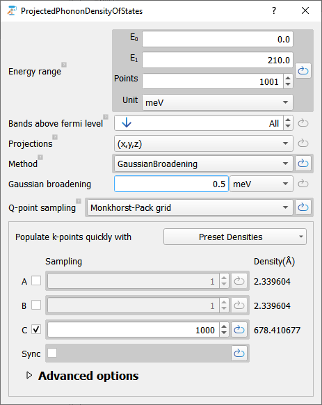
The available projections are

(x,y,z) : Project on (x, y, z) motion of all the atoms. (Default projection type)

Sites : Project on each atom, sum over x,y,z.

Tags : Project on each tag, sum over x,y,z.

Elements : Project on each element, sum over x,y,z.

Sites and (x,y,z) : Project on each atom and x,y,z. This will generate 3*N projection, where N is the number of atoms.

Tags and (x,y,z) : Project on each tag and x,y,z.

Elements and (x,y,z) : Project on each tag and x,y,z.

# %% (6,0) Carbon Nanotube

# Set up lattice
vector_a = [14.700167046094046, 0.0, 0.0]*Angstrom
vector_b = [0.0, 14.700167046094046, 0.0]*Angstrom
vector_c = [0.0, 0.0, 4.26258]*Angstrom
lattice = UnitCell(vector_a, vector_b, vector_c)

# Define elements
elements = [Carbon, Carbon, Carbon, Carbon, Carbon, Carbon, Carbon, Carbon,
            Carbon, Carbon, Carbon, Carbon, Carbon, Carbon, Carbon, Carbon,
            Carbon, Carbon, Carbon, Carbon, Carbon, Carbon, Carbon, Carbon]

# Define coordinates
fractional_coordinates = [[ 0.659867810732,  0.5           ,  0.666666666667],
                          [ 0.638449585341,  0.579933905366,  0.833333333333],
                          [ 0.659867810732,  0.5           ,  0.333333333333],
                          [ 0.579933905366,  0.638449585341,  0.666666666667],
                          [ 0.5           ,  0.659867810732,  0.833333333333],
                          [ 0.638449585341,  0.579933905366,  0.166666666667],
                          [ 0.579933905366,  0.638449585341,  0.333333333333],
                          [ 0.420066094634,  0.638449585341,  0.666666666667],
                          [ 0.361550414659,  0.579933905366,  0.833333333333],
                          [ 0.5           ,  0.659867810732,  0.166666666667],
                          [ 0.420066094634,  0.638449585341,  0.333333333333],
                          [ 0.340132189268,  0.5           ,  0.666666666667],
                          [ 0.361550414659,  0.420066094634,  0.833333333333],
                          [ 0.361550414659,  0.579933905366,  0.166666666667],
                          [ 0.340132189268,  0.5           ,  0.333333333333],
                          [ 0.420066094634,  0.361550414659,  0.666666666667],
                          [ 0.5           ,  0.340132189268,  0.833333333333],
                          [ 0.361550414659,  0.420066094634,  0.166666666667],
                          [ 0.420066094634,  0.361550414659,  0.333333333333],
                          [ 0.579933905366,  0.361550414659,  0.666666666667],
                          [ 0.638449585341,  0.420066094634,  0.833333333333],
                          [ 0.5           ,  0.340132189268,  0.166666666667],
                          [ 0.579933905366,  0.361550414659,  0.333333333333],
                          [ 0.638449585341,  0.420066094634,  0.166666666667]]

# Set up configuration
bulk_configuration = BulkConfiguration(
    bravais_lattice=lattice,
    elements=elements,
    fractional_coordinates=fractional_coordinates
    )


# %% Set ForceFieldCalculator

# %% ForceFieldCalculator
potentialSet = Tersoff_C_2010()
calculator = TremoloXCalculator(parameters=potentialSet)

# %% Set Calculator
bulk_configuration.setCalculator(calculator)
bulk_configuration.update()

# %% OptimizeGeometry
optimized_configuration = OptimizeGeometry(
    configuration=bulk_configuration,
    max_forces=0.01*eV/Angstrom,
    constraints=[
        BravaisLatticeConstraint()
    ],
    trajectory_filename='CNT_results.hdf5'
)

nlsave('CNT_results.hdf5', optimized_configuration)


# %% DynamicalMatrix
dynamical_matrix = DynamicalMatrix(
    configuration=optimized_configuration,
    filename='CNT_results.hdf5',
    object_id='dm',
    calculator=calculator,
    repetitions=(1, 1, 5)
)
dynamical_matrix.update()


# %% ProjectedPhononDensityOfStates
qpoints = MonkhorstPackGrid(
    na=1,
    nb=1,
    nc=1000
)

projectedphonondensityofstates = ProjectedPhononDensityOfStates(
    dynamical_matrix=dynamical_matrix,
    qpoints=qpoints,
    energies=numpy.linspace(0.0, 210.0, 1001)*meV,
    spectrum_method=GaussianBroadening(
        broadening=0.5*meV
    )
)
nlsave('CNT_results.hdf5', projectedphonondensityofstates)

cnt_projected_phonon_dos.py

Analyze results¶

When the calculation has finished the results can be visualized with the Projected DOS analyzer as illustrated below.

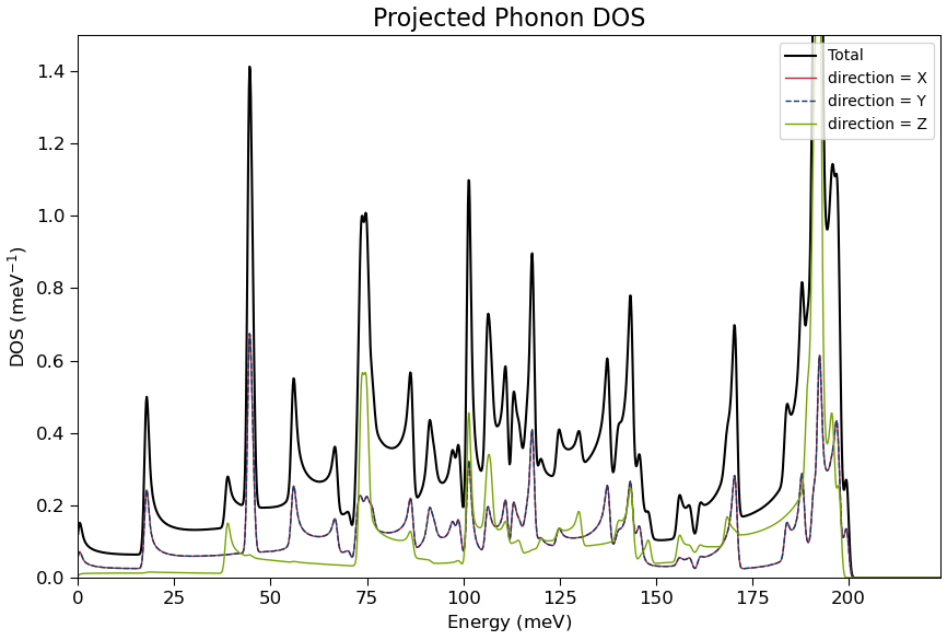
In this case, the projections on x- and y directions are equal due to the rotational symmetry of the CNT. The z-direction movement is, on the other hand significantly different.

Local Phonon Density of States¶

If the PPDOS has been calculated with site projections (Sites or Sites and (x,y,z)), it is possible to plot the phonon density of states as function of spatial coordinates, i.e. the local phonon density of states. This is illustrated in the image below, where the PPDOS is calculated for a SiO2-Si-SiO2 structure as shown in the plot.

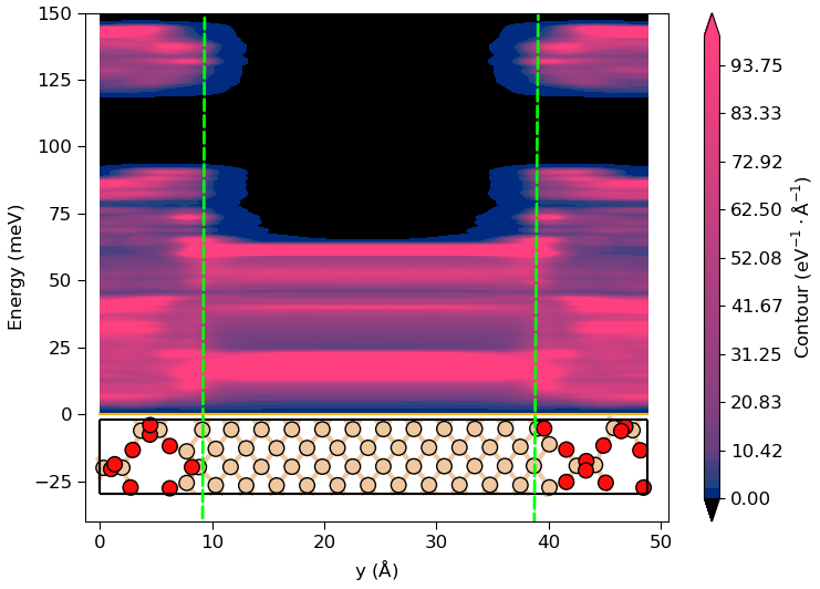
../../../_images/LPDOS-plot-with-structure.png

It is evident that some of the high-energy phonon modes in the SiO2 decays into the central Si region. Such phonon tunneling effects may have important consequences for the phonon-limited mobility in the Si region.