TransmissionPathways
Included in QATK.Analysis
- class TransmissionPathways(configuration=None, energy=None, kpoints=None, contributions=None, self_energy_calculator=None, energy_zero_parameter=None, infinitesimal=None)
Class for representing the Transmission Pathways for a given device configuration and calculator.
- Parameters:
configuration (
DeviceConfiguration) – The device configuration with attached calculator for which the transmission pathways should be calculated.energy (PhysicalQuantity of type energy) – The energy for which the transmission pathway should be calculated. Default:
0.0*eVkpoints (sequence (size 3) of int |
MonkhorstPackGrid|KpointDensity) – The k-points for which the transmission pathways should be calculated. Note that the k-points must be in the xy-plane. Default:MonkhorstPackGrid(na, nb)where(na, nb)is the sampling used for the self-consistent calculation.contributions (
Left|Right) – The transmission pathways contributions from the left or right electrode. Default:Leftself_energy_calculator (
RecursionSelfEnergy|SparseRecursionSelfEnergy) – The self energy calculator to be used for the transmission pathways. Default:RecursionSelfEnergy(storage_strategy=NoStorage())energy_zero_parameter (
AverageFermiLevel|AbsoluteEnergy.) – Specifies the choice for the energy zero. Default:AverageFermiLevelinfinitesimal (PhysicalQuantity of type energy.) – Small positive energy, used to move the transmission calculation away from the real axis. This is only relevant for recursion-style self-energy calculators. Default:
1.0e-6*eV
- electrodeFermiLevels()
- Returns:
The left and right electrodes Fermi levels in absolute energies.
- Return type:
- energy()
- Returns:
The energy used in this transmission pathways.
- Return type:
PhysicalQuantity of type energy
- energyZero()
- Returns:
The energy zero value.
- Return type:
PhysicalQuantity of type energy
- evaluate(spin=None)
Return the atom transmission pathways.
- Parameters:
spin (
Spin.Up|Spin.Down|Spin.Sum|Spin.X|Spin.Y|Spin.Z|Spin.UpUp|Spin.DownDown|Spin.RealUpDown|Spin.ImagUpDown) – The spin used in the analysis Default:Spin.Sum- Returns:
A list with transmission pathway data for the give spin type. Each entry in the list contains the data (atom index i, neighbour atom index j, repetitions, t_ij), where repetitions=(n_A, n_B, n_C) is the repetitions of the neighbour atom in directions A, B, C, and t_ij is the local bond transmission from i to j.
- Return type:
list
- infinitesimal()
- Returns:
The infinitesimal used for calculating the transmission pathways.
- Return type:
PhysicalQuantity of type energy
- metatext()
- Returns:
The metatext of the object or None if no metatext is present.
- Return type:
str | None
- nlinfo()
Returns information about the transmission pathways analysis.
- Returns:
A dictionary containing the analysis information.
- Return type:
dict
- nlprint(stream=None)
Print a string containing an ASCII table useful for plotting the AnalysisSpin object.
- Parameters:
stream (python stream) – The stream the table should be written to. Default:
NLPrintLogger()
- setMetatext(metatext)
Set a given metatext string on the object.
- Parameters:
metatext (str | None) – The metatext string to set. Use “None” to remove current metatext.
- uniqueString()
Return a unique string representing the state of the object.
Usage Examples
Calculate the TransmissionPathways for a device configuration, print out the result, and save them for visualization with QuantumATK:
pathways = TransmissionPathways(device_configuration)
nlprint(pathways)
nlsave('pathways.hdf5', pathways)
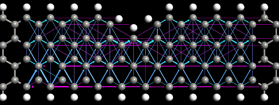
Fig. 197 Spin up component of the transmission pathways of a graphene ribbon with a wedge. Arrows point in the direction of the pathways.The magnitude of the pathway is illustrated by the volume of the arrow and the color shows the direction, i.e. right point arrows are blue and left pointing arrows violet.
Check, that the pathways sum up to the correct transmission spectrum:
pathways = TransmissionPathways(device_configuration)
border_atom = len(device_configuration.elements())/2
print 'transmission coefficient ',
print pathways._transmissionCoefficient(border_atom=border_atom)
Notes
The TransmissionPathways is an analysis option which splits the transmission coefficient into local bond contributions, \(T_{ij}\). The pathways have the property that if the system is divided into 2 parts (\(A,B\)), then the pathways across the boundary between \(A\) and \(B\) sum up to the total transmission coefficient
The local bond contributions, \(T_{ij}\) , can be both positive and negative. A negative value correspond to that the electron is back scattered along the bond. A positive value of \(T_{ij}\) is visualized as an arrow from \(i\) to \(j\) while a negative value is visualized as an arrow from \(j\) to \(i\), i.e. the direction of the arrows shows the flow of the electrons.
For further details, see [1].