calculateNonSelfConsistentFiniteBiasSpinTransferTorque

calculateNonSelfConsistentFiniteBiasSpinTransferTorque(configuration, biases, potential_drop_region=None, potential_profile=None, kpoints=None)

Calculate the atom-resolved spin transfer torque at finite bias, within a non-selfconsistent approximation for the non equilibrium potential.

The non-equilibrium potential is modelled as a ramp as specified in the parameter potential_drop_region, or as a user-defined piecewise function as defined in potential_profile.

Parameters:

• configuration (DeviceConfiguration.) – The configuration to calculate the spin torque transfer torkance. The configuration must have a calculator with non-collinear spin.

• biases – A list of the bias voltages for which the torque should be calculated.
  Default: [0.1] * Volt

• potential_drop_region (A list of integers or a list of PhysicalQuantity of type position.) – Defines the potential model as a linear ramp, where the potential drop occurs in a spatial region specified by the input parameters. The parameters can be either the first and last atom where the potential drop occurs, or the initial and final coordinates along the C axis for the potential ramp. In an Magnetic Tunneling Junction geometry, the indices or the z coordinates of the metal atoms at the interface with the insulating barrier should be used. This argument is mutually exclusive to potential_profile.

• potential_profile (List of (PhysicalQuantity of type length, float)) –

  Defines the potential model as a piecewise linear function, defined as a list of (coordinate, value) pairs, where the values define the potential drop in an interval \((+V_b/2, V_b/2)\) with \(V_b\) the applied bias.

  For example, a list [(0*Ang, 1), (5*Ang, 1), (10*Ang, 0.), (15*Ang, 0.), (20*Ang, -1.), (25*Ang, -1.)] represents a potential ramp from \(V_b/2\) to \(-V_b/2\) between coordinates 5 and 20 Angstrom, with a flat 0 potential region in the middle. It is required that the leftmost and rightmost values are 1 and -1 respectively.

  This parameter is mutually exclusive to potential_drop_region and can be used to define more complex potential drop profiles than a single ramp, e.g. in presence multiple tunneling barriers.

• kpoints (sequence (size 3) of int | MonkhorstPackGrid | KpointDensity) – The k-points for which the spin transfer torque should be calculated.
  Default: The Monkhorst-Pack grid used for the self-consistent calculation.

Returns:

A tuple with the total torque per bias point, the torque per k-point and bias point, the k-points and weights used for the integration.

Return type:

A tuple (torque, torque_per_kpoint, kpoints, weights) where torque and torque_per_kpoint are a list of PhysicalQuantity of type energy of size (3, natoms) and (3, natoms, nk) per each bias point.

Usage Examples

In this example we will calculate the spin transfer torque (STT) in a a Fe-MgO-Fe magnetic tunneling junction (MTJ) for an angle of 90 degree between the magnetization in the fixed (left) and free (right) magnetic regions.

As starting point, we define the configuration and calculate the solution for a parallel spin configuration.

# -*- coding: utf-8 -*-
# -------------------------------------------------------------
# Two-probe Configuration
# -------------------------------------------------------------
# -------------------------------------------------------------
# Left Electrode
# -------------------------------------------------------------

# Set up lattice
vector_a = [2.866, 0.0, 0.0]*Angstrom
vector_b = [0.0, 2.866, 0.0]*Angstrom
vector_c = [0.0, 0.0, 2.866]*Angstrom
left_electrode_lattice = UnitCell(vector_a, vector_b, vector_c)

# Define elements
left_electrode_elements = [Iron, Iron]

# Define coordinates
left_electrode_coordinates = [[ 0.7165,  0.7165,  0.7165],
                              [ 2.1495,  2.1495,  2.1495]]*Angstrom

# Set up configuration
left_electrode = BulkConfiguration(
    bravais_lattice=left_electrode_lattice,
    elements=left_electrode_elements,
    cartesian_coordinates=left_electrode_coordinates
    )

# -------------------------------------------------------------
# Right Electrode
# -------------------------------------------------------------

# Set up lattice
vector_a = [2.866, 0.0, 0.0]*Angstrom
vector_b = [0.0, 2.866, 0.0]*Angstrom
vector_c = [0.0, 0.0, 2.866]*Angstrom
right_electrode_lattice = UnitCell(vector_a, vector_b, vector_c)

# Define elements
right_electrode_elements = [Iron, Iron]

# Define coordinates
right_electrode_coordinates = [[ 2.1495,  2.1495,  0.7165],
                               [ 0.7165,  0.7165,  2.1495]]*Angstrom

# Set up configuration
right_electrode = BulkConfiguration(
    bravais_lattice=right_electrode_lattice,
    elements=right_electrode_elements,
    cartesian_coordinates=right_electrode_coordinates
    )

# -------------------------------------------------------------
# Central Region
# -------------------------------------------------------------

# Set up lattice
vector_a = [2.866, 0.0, 0.0]*Angstrom
vector_b = [0.0, 2.866, 0.0]*Angstrom
vector_c = [0.0, 0.0, 39.06710000000001]*Angstrom
central_region_lattice = UnitCell(vector_a, vector_b, vector_c)

# Define elements
central_region_elements = [Iron, Iron, Iron, Iron, Iron, Iron, Iron, Iron, Magnesium, Oxygen,
                           Oxygen, Magnesium, Magnesium, Oxygen, Oxygen, Magnesium, Magnesium,
                           Oxygen, Oxygen, Magnesium, Magnesium, Oxygen, Iron, Iron, Iron,
                           Iron, Iron, Iron, Iron, Iron]

# Define coordinates
central_region_coordinates = [[  0.7165 ,   0.7165 ,   0.7165 ],
                              [  2.1495 ,   2.1495 ,   2.1495 ],
                              [  0.7165 ,   0.7165 ,   3.5825 ],
                              [  2.1495 ,   2.1495 ,   5.0155 ],
                              [  0.7165 ,   0.7165 ,   6.4485 ],
                              [  2.1495 ,   2.1495 ,   7.8815 ],
                              [  0.7165 ,   0.7165 ,   9.3145 ],
                              [  2.1495 ,   2.1495 ,  10.7475 ],
                              [  0.7165 ,   0.7165 ,  12.9475 ],
                              [  2.1495 ,   2.1495 ,  12.9475 ],
                              [  0.7165 ,   0.7165 ,  15.14285],
                              [  2.1495 ,   2.1495 ,  15.14285],
                              [  0.7165 ,   0.7165 ,  17.3382 ],
                              [  2.1495 ,   2.1495 ,  17.3382 ],
                              [  0.7165 ,   0.7165 ,  19.53355],
                              [  2.1495 ,   2.1495 ,  19.53355],
                              [  0.7165 ,   0.7165 ,  21.7289 ],
                              [  2.1495 ,   2.1495 ,  21.7289 ],
                              [  0.7165 ,   0.7165 ,  23.92425],
                              [  2.1495 ,   2.1495 ,  23.92425],
                              [  0.7165 ,   0.7165 ,  26.1196 ],
                              [  2.1495 ,   2.1495 ,  26.1196 ],
                              [  2.1495 ,   2.1495 ,  28.3196 ],
                              [  0.7165 ,   0.7165 ,  29.7526 ],
                              [  2.1495 ,   2.1495 ,  31.1856 ],
                              [  0.7165 ,   0.7165 ,  32.6186 ],
                              [  2.1495 ,   2.1495 ,  34.0516 ],
                              [  0.7165 ,   0.7165 ,  35.4846 ],
                              [  2.1495 ,   2.1495 ,  36.9176 ],
                              [  0.7165 ,   0.7165 ,  38.3506 ]]*Angstrom

# Set up configuration
central_region = BulkConfiguration(
    bravais_lattice=central_region_lattice,
    elements=central_region_elements,
    cartesian_coordinates=central_region_coordinates
    )

device_configuration = DeviceConfiguration(
    central_region,
    [left_electrode, right_electrode],
    equivalent_electrode_lengths=[5.732, 5.732]*Angstrom,
    transverse_electrode_repetitions=[[1, 1], [1, 1]],
    )

# -------------------------------------------------------------
# Calculator
# -------------------------------------------------------------
#----------------------------------------
# Basis Set
#----------------------------------------
basis_set = [
    LDABasis.Oxygen_SingleZeta,
    LDABasis.Iron_SingleZetaPolarized,
    LDABasis.Magnesium_SingleZetaPolarized,
    ]

#----------------------------------------
# Exchange-Correlation
#----------------------------------------
exchange_correlation = LSDA.PZ

#----------------------------------------
# Numerical Accuracy Settings
#----------------------------------------
device_k_point_sampling = MonkhorstPackGrid(
    na=21,
    nb=21,
    nc=300,)
device_numerical_accuracy_parameters = NumericalAccuracyParameters(
    k_point_sampling=device_k_point_sampling,
    )

#----------------------------------------
# Contour Integral Settings
#----------------------------------------
equilibrium_contour = SemiCircleContour(
    integral_lower_bound=2.55775293896*Hartree,
    )

contour_parameters = ContourParameters(
    equilibrium_contour=equilibrium_contour,
    )

device_algorithm_parameters = DeviceAlgorithmParameters(
    initial_density_type=EquivalentBulk(electrode_constraint_length=3.*Ang)
    )

#----------------------------------------
# Device Calculator
#----------------------------------------
calculator = DeviceLCAOCalculator(
    basis_set=basis_set,
    exchange_correlation=exchange_correlation,
    numerical_accuracy_parameters=device_numerical_accuracy_parameters,
    contour_parameters=contour_parameters,
    device_algorithm_parameters=device_algorithm_parameters,
    )

device_configuration.setCalculator(calculator)

# -------------------------------------------------------------
# Initial State
# -------------------------------------------------------------
scaled_spins = [1] * 8 + [0] * 14 + [1] * 8
initial_spin = InitialSpin(scaled_spins=scaled_spins)

device_configuration.setCalculator(
    calculator,
    initial_spin=initial_spin,
)
device_configuration.update()
filename = 'polarized-0.hdf5'
nlsave(filename, device_configuration)

0-polarized.py

In order to calculate the STT, we need to rotate the spin in the free layer to obtain the desired magnetization direction. We apply a spin rotation to the previously calculated solution for the parallel configuration. Since we are only changing the magnetization direction, we can perform a non-selfconsistent update.

Note

For numerical reasons, the torque components are best determined in the layer with spin orientation along z, therefore it is suggested to rotate the spin in the fixed layer as in this example.

With this configuration we calculate the finite bias STT in a bias interval from -1 to 1 Volt, and for sake of comparison we also calculate the atom-resolved torkance. These steps are performed in the script below.

# Apply a spin rotation on top of the Polarized collinear solution and
# update non-selfconsistently.
device_configuration = nlread('polarized-0.hdf5', DeviceConfiguration)[-1]
calculator = device_configuration.calculator()
exchange_correlation = NCLDA.PZ
calculator = calculator(
    exchange_correlation=exchange_correlation,
    iteration_control_parameters=NonSelfconsistent
    )

# -------------------------------------------------------------
# Initial State
# -------------------------------------------------------------
# Define the spin rotation in polar coordinates
theta = 90
left_spins  = [(i, 1, theta * Degrees, 0 * Degrees) for i in range(8)]
center_spins  = [(i, 0, 0 * Degrees, 0 * Degrees) for i in range(8, 22)]
right_spins = [(i, 1, 0 * Degrees, 0 * Degrees) for i in range(22, 30)]
spin_list   = left_spins + center_spins + right_spins
initial_spin = InitialSpin(scaled_spins=spin_list)
device_configuration.setCalculator(
    calculator,
    initial_spin=initial_spin,
    initial_state=device_configuration
)

# Update and save.
device_configuration.update()
filename = 'theta-{}.hdf5'.format(theta)
nlsave(filename, device_configuration)

# Calculate and save the atom-resolved torkance.
torkance, torkance_per_kpoint, kpoints, weights = calculateLinearResponseSpinTransferTorkance(
    device_configuration)
nlsave('stt-90.hdf5', torkance, object_id='torkance')

# Calculate and save the finite bias torque in a bias range of interest.
biases = numpy.linspace(-1.0, 1.0, 21) * Volt
torque, torque_per_kpoint, kpoints, weights = calculateNonSelfConsistentFiniteBiasSpinTransferTorque(
    configuration=device_configuration,
    biases=biases,
    potential_drop_region=(7, 22))
nlsave('stt-90.hdf5', torque, object_id='torque')
nlsave('stt-90.hdf5', biases, object_id='biases')

finite_bias_stt.py

With the script below we can visualize the total torque integrated in the free layer and compare the atom-resolved torque with the linear response torkance, evaluated using calculateLinearResponseSpinTransferTorkance.

from matplotlib import pyplot as plt

# Unit conversion from eV to uJ/m^2
surface = 2.866 * 2.866 * 1e-20 # in m * m
conversion = (1 * eV).inUnitsOf(Joule) * 1e6 / surface

filename = 'stt-90.hdf5'
initial_free_layer_site = 22

# Retrieve the saved quantities
torkance_linear_response = nlread(filename, object_id='torkance')[0]
torque = nlread(filename, object_id='torque')[0]
biases = nlread(filename, object_id='biases')[0]

# Plot the torque obtained from the linear repsonse torkance.
total_torkance = numpy.sum(torkance_linear_response[:, initial_free_layer_site:], axis=1)
torque_from_torkance_x = [- total_torkance[0] * bias * conversion for bias in biases.inUnitsOf(Volt)]
plt.plot(biases, torque_from_torkance_x, '--', label='In-plane torque (linear response)')

total_torque_x = [numpy.sum(x[0, initial_free_layer_site:]) * conversion for x in torque.inUnitsOf(eV)]
plt.plot(biases, total_torque_x, 'o-', linewidth=2, label='In-plane torque (finite bias)')

total_torque_y = [numpy.sum(x[1, initial_free_layer_site:]) * conversion for x in torque.inUnitsOf(eV)]
plt.plot(biases, total_torque_y, 'o-', linewidth=2, label='Out-of-plane torque (finite bias)')

plt.xlabel('Voltage [V]')
plt.ylabel('Torque [uJ/m^2]')
plt.title(r'$\theta = \pi/2$')
plt.legend()
plt.grid()
plt.show()

# Plot the torque per atomic site.
single_bias_point = - 0.6
idx = 4

plt.plot(- single_bias_point * torkance_linear_response[0, :] * conversion, 'o--', label='In-plane torque (linear response)')
plt.plot(torque.inUnitsOf(eV)[idx][0, :] * conversion, '*-', label='In-plane torque (finite bias)')

plt.title('Torque at {} V'.format(single_bias_point))
plt.ylabel('Torque [uJ/m^2]')
plt.xlabel('Atom no.')
plt.legend()
plt.grid()
plt.show()

plot.py

Results are shown in the figures below.

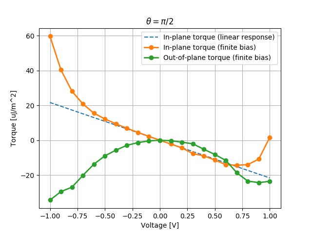
Fig. 176 Total Spin Transfer Torque integrated in the right metallic layer.

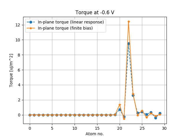
Fig. 177 Atom-resolved Spin Transfer Torque at -0.6 Volt evaluated with the finite bias and with the linear response methods.

The non-linear behavior of the in-plane component for large bias and the quadratic behavior of the out-of-plane component are consistent with literature results [1], [2].

This example runs in about 240 core-hours on a modern HPC cluster, with quite loose numerical parameters. Wallclock time can be dramatically reduced by massive parallelization, since this kind of calculation scales well.

Note

Results are very sensitive to numerical parameters such as k-point sampling or real axis contour accuracy. Convergence with respect to those parameters should be carefully checked.

Note that the non-equilibrium contour parameters used to evaluate the density matrix (see ContourParameters) are taken from the calculator attached to the input configuration.

Notes

The spin transfer torque is evaluated in a non-selfconsistent finite bias approximation. The potential drop across the barrier is represented as a ramp across the tunneling barrier [2], avoiding time consuming and often hard to converge non-collinear calculations at finite bias. To best approximate the finite-bias potential, the potential ramp must be defined in between the metal atoms at the interface (included).

The atom-resolved torque on an atom \(a\) is then calculated as [3] :

\[\mathbf{T}_{CD, a} = \sum_{\alpha \in a} \sum_{\beta} \Re [\rho_{CD, \alpha \beta} \mathbf{\sigma} \times \mathbf{B}_{XC, \alpha \beta}]\]

where \(\rho_{CD} = \rho_{neq} - \rho_{eq}\) is the current driven density matrix, given by the difference between the density matrix at finite bias and at equilibrium.

[1]

Xingtao Jia, Ke Xia, Youqi Ke, and Hong Guo. Nonlinear bias dependence of spin-transfer torque from atomic first principles. Phys. Rev. B, 84:014401, Jul 2011. URL: https://link.aps.org/doi/10.1103/PhysRevB.84.014401, doi:10.1103/PhysRevB.84.014401.

[2] (1,2)

Ivan Rungger, Andrea Droghetti, and Maria Stamenova. Non-equilibrium Green’s Function Methods for Spin Transport and Dynamics, pages 1–27. Springer International Publishing, Cham, 2018. URL: https://doi.org/10.1007/978-3-319-42913-7_75-1, doi:10.1007/978-3-319-42913-7_75-1.

[3]

Branislav K. Nikolic, Kapildeb Dolui, Marko D. Petrovic, Petr Plechac, Troels Markussen, and Kurt Stokbro. First-Principles Quantum Transport Modeling of Spin-Transfer and Spin-Orbit Torques in Magnetic Multilayers, pages 1–35. Springer International Publishing, Cham, 2018. URL: https://doi.org/10.1007/978-3-319-50257-1_112-1, doi:10.1007/978-3-319-50257-1_112-1.