Battery Open Circuit Voltage (OCV) Prediction for Lithium-Ion Cathode Materials

This application demonstrates how to calculate Open Circuit Voltage (OCV) curves for lithium-ion battery cathode materials as a function of lithiation level. The workflow samples multiple lithium/vacancy orderings at each composition, performs geometry optimization, and computes voltage profiles from total energies.

Important

QuantumATK Version: This application is designed for QuantumATK X-2025.06-SP1.

The scripts support both Machine Learning Force Fields (MLFF) and DFT calculators. Download the example files below:

• ocv_vs_lithiation_NMC.py - OCV calculation for NMC cathodes

• ocv_vs_lithiation_LFP.py - OCV calculation for LiFePO₄

• configuration.py - Structure definitions for Li metal, FePO₄, LiFePO₄

• config_NMC.py - NMC cathode structure generator

• DFTcalculator.py - DFT calculator setup (optional)

Key Features

• Multiple cathode chemistries: Nickel-Manganese-Cobalt oxide or NMC (811, 721, 622, 532) and LiFePO₄ or LFP

• Configurational sampling: Systematic generation of Li/vacancy orderings using clustered, uniform, and random patterns

• Ground state identification: Automatic selection of lowest-energy configuration at each lithiation level

• Flexible calculators: Switch between fast MLFF (MatterSim) and accurate DFT (HSE06)

Theoretical Background: What is OCV?

Open Circuit Voltage (OCV) Fundamentals

OCV Illustration

Fig. 136 OCV calculation concept: The voltage is derived from the energy difference between lithiated and delithiated cathode states relative to metallic lithium reference.

The Open Circuit Voltage (OCV) is the equilibrium voltage of a battery when no current flows through the cell. It represents the thermodynamic driving force for the electrochemical reaction and is a fundamental property that determines battery performance characteristics including:

• Energy density: Total energy stored per unit mass or volume

• Power capability: Maximum discharge/charge rates

• State of charge (SOC): Relationship between voltage and remaining capacity

• Cycling stability: Voltage fade and capacity retention over charge-discharge cycles

For a lithium-ion battery, the overall cell voltage is determined by the difference in chemical potential of lithium between the cathode and anode materials.

Thermodynamic Basis

Fundamentally, the cell voltage is determined by the change in Gibbs free energy with respect to lithium content, which equals the difference in the chemical potential of lithium (\(\mu_{\text{Li}}\)) between the cathode and the anode:

\[V(x) = -\frac{1}{e}\frac{\partial G}{\partial x} = -\frac{\mu_{\text{Li}}^{\text{cathode}}(x) - \mu_{\text{Li}}^{\text{anode}}}{e}\]

Where \(x\) represents the lithium concentration in the host material \(\text{Li}_x\text{Host}\), \(G\) is the Gibbs free energy, and \(e\) is the elementary charge.

In computational practice at 0 K, we approximate the Gibbs free energy (\(G\)) simply as the internal total energy (\(E\)), neglecting entropic contributions (\(-TS\)).

Computational Approach: The Difference Method

To calculate OCV, we compare the total energies of cathode (host) and anode (Li source) supercells at distinct lithiation fractions. The average voltage between two compositions \(x_1\) and \(x_2\) (where \(x_2 > x_1\)) is given by:

\[V \approx \frac{-\left[ E(\text{Li}_{x_2}\text{Host}) - E(\text{Li}_{x_1}\text{Host}) - (n_2 - n_1) E_{\text{Li}}^{\text{bulk}} \right]}{n_2 - n_1}\]

where:

• \(E(\text{Li}_{x}\text{Host})\) is the total energy of the cathode supercell at concentration \(x\) (eV).

• \(n\) is the integer number of Lithium atoms in the supercell.

• \(E_{\text{Li}}^{\text{bulk}}\) is the energy per atom of metallic Lithium (anode reference) (eV).

• \(n_2 - n_1\) is the number of Lithium atoms added during the step.

Note

The negative sign ensures that if the lithiation is exothermic (\(E_{final} < E_{initial}\)), the resulting voltage is positive.

Key approximations:

• Zero temperature (0 K): Uses electronic ground state energies only

• Sampling strategy: Finite number of samples may fail to capture ground states

• Nernstian voltage calculation: Voltage is derived from the finite differences. This produces average voltages over an interval, contributing to “staircase” visual artefact

• Thermodynamic approximation: Neglects kinetics of charging/discharging and any effects of nonequilibrium conditions

Why Computational OCV Prediction is Valuable

Computational OCV prediction enables:

• Rapid materials screening: Evaluate thousands of candidates before synthesis

• Structure-property insight: Link atomic structure to voltage, stability, and cycling performance

• Experimental guidance: Resolve ambiguities and predict behavior at extreme conditions

• Cost efficiency: MLFF (hours-days) or DFT (days-weeks) vs. months of lab optimization

System Overview

This application addresses two major cathode material families:

1. Layered NMC (LiNi_aMn_bCo_cO₂)

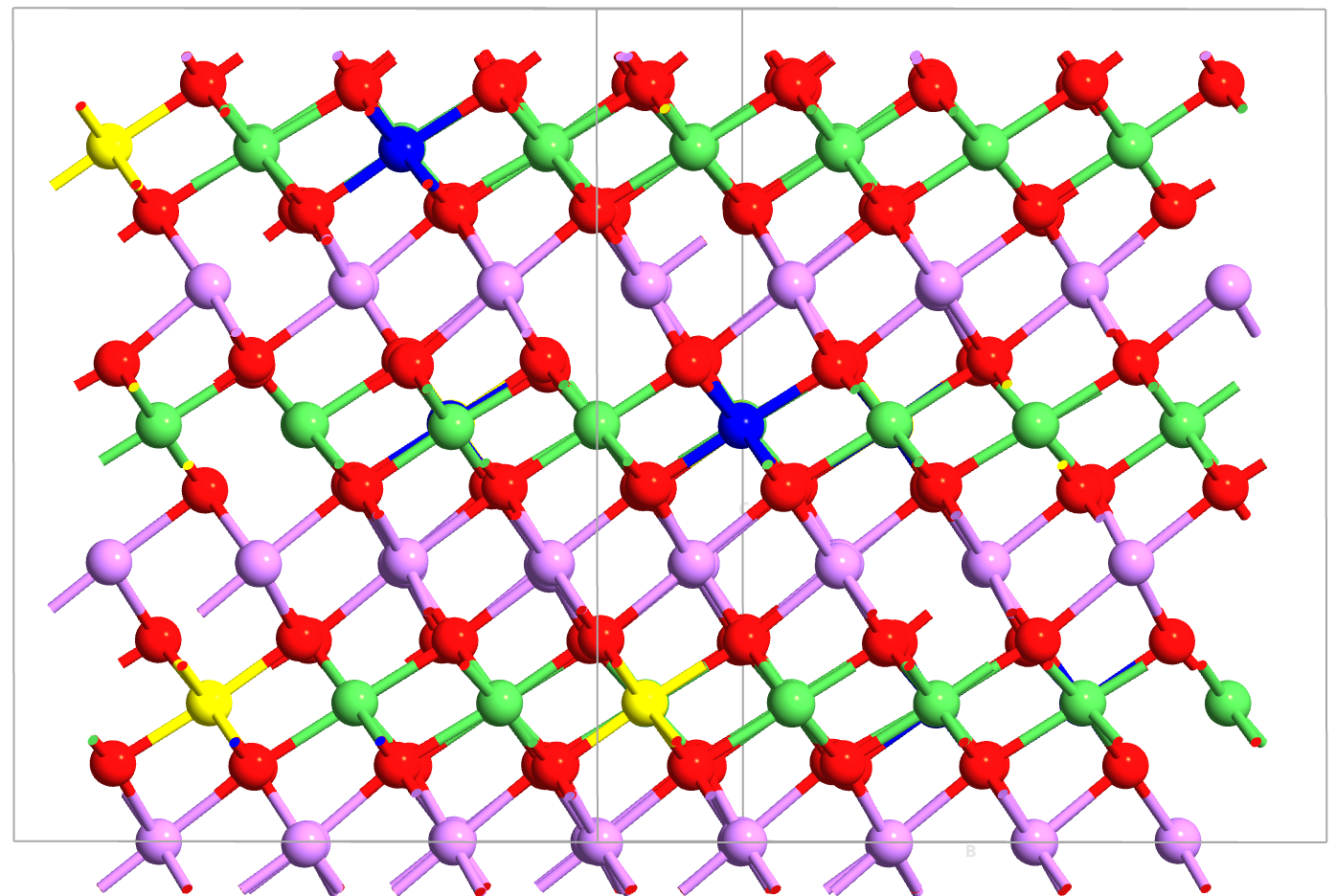
Fig. 137 NMC layered structure. Li ions (lavender) occupy 2D layers between transition metal (TM) oxide slabs (Ni/Mn/Co shown in green/yellow/blue). The TM sublattice exhibits random mixing requiring Special Quasi-random Structure (SQS) modeling.

• Structure: Layered rock-salt (R-3m space group) with Li⁺ in octahedral sites between TM-O layers

• Compositions: NMC811 (Ni₀.₈Mn₀.₁Co₀.₁O₂), NMC721, NMC622, NMC532

• Applications: High-energy density electric vehicle batteries

• Voltage range: Typically 3.6-4.3 V vs Li/Li⁺ (sloped profile) [1]

• Characteristics: solid-solution behavior, requires SQS for TM disorder

2. Olivine LiFePO₄ (LFP)

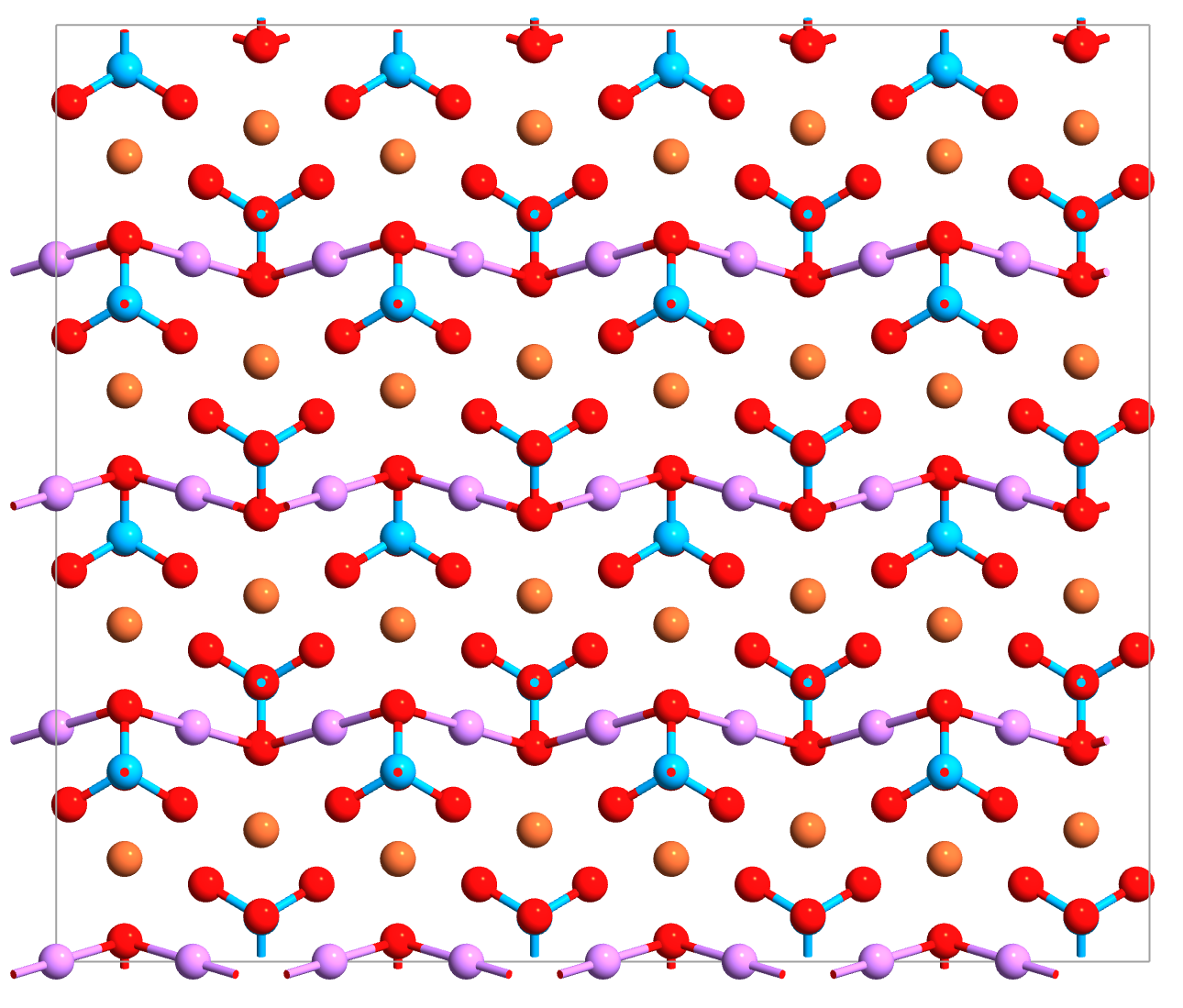
Fig. 138 LiFePO₄ olivine structure. Li ions (lavender) occupy 1D channels parallel to the b-axis. Fe sites (brown) are crystallographically ordered, unlike the random TM distribution in NMC.

• Structure: Orthorhombic olivine (Pnma space group) with 1D Li diffusion channels

• Applications: Safe, long-cycle-life batteries for EVs and grid storage

• Voltage range: Dominated by a flat plateau at ~3.3–3.45 V vs Li/Li⁺ [2][3]

• Characteristics: Two-phase coexistence (LiFePO₄ ↔ FePO₄) during (de)lithiation, ordered Fe sites

Key Computational Differences:

Aspect	LiFePO₄	NMC
TM sublattice	Ordered Fe sites (crystallographic)	Random Ni/Mn/Co mixing (requires SQS)
Li sublattice	1D channels	2D interlayer sites
Simulation approach	Add Li to empty FePO₄ (bottom-up)	Remove Li from full Li₁NMC (top-down)
Starting structures	Two templates (FePO₄ + LiFePO₄)	Single SQS supercell
Phase behavior	Two-phase (flat voltage plateau)	Solid solution (sloped voltage curve)

The simulation workflow for NMC systematically removes lithium atoms from the fully lithiated SQS structure to simulate progressive delithiation. For LiFePO₄, lithium atoms are systematically added to the empty FePO₄ framework. In both cases, energies at each composition are computed and voltages derived from total energy differences.

Simulation Workflow

The OCV calculation follows a systematic workflow: prepare cathode structures at different lithiation levels, optimize geometries, compute energies, and extract voltage profiles. The main difference between materials is how structures are prepared (NMC requires SQS for disorder, LFP uses crystallographic templates).

Inputs and Configuration

Structure preparation:

• NMC: Composition fractions (NI_FRAC=0.6, MN_FRAC=0.2, CO_FRAC=0.2), supercell size (REPEAT_A=5, REPEAT_B=4, REPEAT_C=1), SQS parameters (SQS_GENERATIONS=150, SQS_POPULATION_SIZE=100, CLUSTER_MAX_DIAMETERS), Mn/Co splitting method (SPLIT_METHOD='random' or 'fps'), optimization settings (MAX_FORCES=0.01*eV/Angstrom, OPTIMIZE_CELL=True)

• LFP: Primitive cell structures from configuration.py (FePO4(), LiFePO4(), Li_metal4()), supercell repetition (repeat_cells = (2, 4, 1))

Sampling and optimization:

• NMC: Composition grid x_target = numpy.linspace(0.0, 1.0, 21) (user-configurable, 21 points default), cell relaxation toggle OPTIMIZE_CELL = True

• LFP: Composition grid auto-generated for all integer Li counts with optional subsampling factor k=2, cell relaxation always enabled

• Sampling intensity: n_samples_per_x = 150 (1 clustered + 1 uniform + 148 random)

• Calculator: CALCULATOR = 'MATTERSIM' (fast) or 'DFT' (accurate)

• Optimization: force convergence max_forces = 0.01*eV/Angstrom, maximum steps max_steps = 1000

Note

Customization: Adjust x_target (NMC) to control composition grid spacing (11 points for fast screening, 41 for smooth curves). Modify n_samples_per_x to balance computational cost vs. ground state accuracy (10 = fast, 150 = standard, 500 = exhaustive).

Overview of Computational Steps

For NMC cathodes (top-down delithiation):

1. Preprocessing: Generate SQS structure to model Ni/Mn/Co disorder → config_NMC.py

2. Main calculation: Load SQS, systematically remove Li atoms, find ground states → ocv_vs_lithiation_NMC.py

For LiFePO₄ (bottom-up lithiation):

1. Main calculation: Start from empty FePO₄, systematically add Li atoms, find ground states → ocv_vs_lithiation_LFP.py

Both calculations compute Li metal reference energy and derive voltages from total energy differences.

Step 1: Structure Preparation

NMC: Special Quasi-random Structure (SQS) Generation

Since NMC cathodes have randomly mixed Ni/Mn/Co atoms on the transition metal sublattice, you must first generate a disordered supercell that statistically represents this mixing using config_NMC.py. The script uses a binary SQS workaround to handle ternary NMC alloys: it creates a supercell from the layered LiCoO₂ primitive cell, sets up a binary alloy (Ni vs. “X” where X = Mn+Co combined using Zn as placeholder), runs an evolutionary SQS algorithm to generate statistically random Ni/X distribution, then splits X atoms into Mn and Co proportionally (random or FPS distribution). Finally, the geometry is optimized with cell relaxation. This preprocessing is performed once per composition (NMC811, NMC721, NMC622, NMC532), and the resulting SQS file is used as input for the OCV calculation script.

LiFePO₄: Direct Structure Loading

LFP has ordered Fe sites, so no SQS is needed. The script loads crystallographic structure definitions from configuration.py and repeats the FePO₄ and LiFePO₄ primitive cells to the desired supercell size (e.g., repeat_cells = (2, 4, 1) creates 32 Li sites). Li site positions are extracted from the LiFePO₄ template to define where lithium can be added, while FePO₄ serves as the empty host framework for bottom-up lithiation. The Li metal structure is also loaded for reference energy calculation. These three structure templates (FePO₄, LiFePO₄, Li metal supercells) remain in memory with no file output at this stage.

Step 2: Configurational Sampling

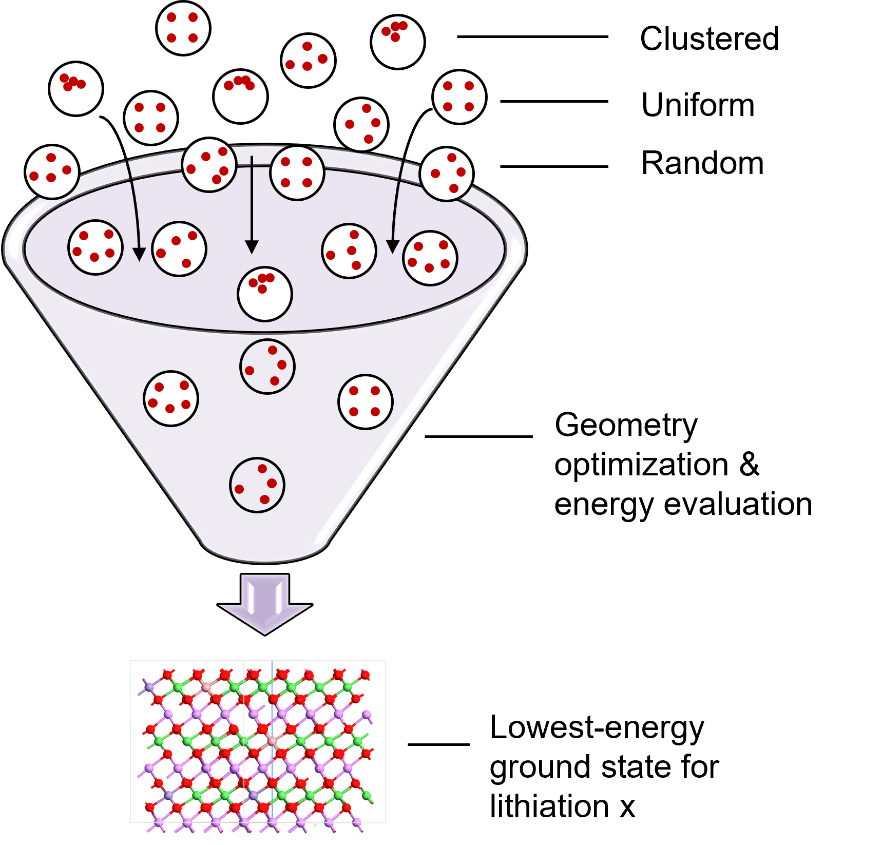
Fig. 139 Three sampling strategies explore different Li/vacancy arrangements to find the lowest-energy (ground state) configuration at each composition.

At each lithiation level x, the script generates many candidate structures with different Li/vacancy arrangements using three strategies: clustered (Li atoms/vacancies concentrated in one region), uniform (Farthest-Point Sampling with maximal spreading), and random (statistical exploration of configuration space). For NMC, the script starts with the fully lithiated SQS and removes Li atoms according to each strategy; for LFP, it starts with empty FePO₄ and adds Li atoms. This generates 150 candidate structures per composition point (1 clustered + 1 uniform + 148 random), all inheriting the transition metal arrangement from the SQS (NMC) or ordered Fe sites (LFP). The candidate configurations are stored in memory for subsequent optimization.

Step 3: Energy Calculation and Ground State Identification

Each candidate configuration is geometry-optimized and its total energy computed to identify the lowest-energy (ground state) configuration at each composition. For each of the ~150 candidates per composition, the script attaches the selected calculator (MatterSim-5M MLFF or HSE06 DFT), optimizes atomic positions and lattice parameters until forces converge below 0.01 eV/Å, computes the total energy, and compares all energies to select the ground state.

Note

MatterSim-5M MLFF is the default and recommended calculator because it is 100-1000× faster than DFT, enabling extensive configurational sampling (150 candidates per composition) that would be computationally prohibitive with DFT. For final validation or when highest accuracy is required, HSE06 DFT (requires DFTcalculator.py) can be used on a reduced set of ground state structures.

Step 4: Li Metal Reference Energy

To compute voltage vs. Li/Li⁺, the script calculates the energy of bulk lithium metal as a reference state. The Li metal structure (BCC, from Li_metal4() in configuration.py) undergoes geometry optimization including cell shape and volume relaxation, followed by total energy calculation. The resulting energy is divided by the number of Li atoms to obtain the energy per atom (E_Li), which serves as the chemical potential reference for voltage calculations.

Step 5: Voltage Calculation

Voltages are computed from finite differences in energy between adjacent compositions using the ground state energies, Li atom counts, and Li metal reference energy. For each pair of adjacent compositions, the script calculates the energy difference between the two configurations, subtracts the Li metal contribution to obtain the reaction energy, divides by the number of Li atoms transferred to get the voltage, and assigns this voltage value to the midpoint composition between the two states. This finite-difference approach produces the characteristic staircase voltage profile.

Step 6: Results Visualization

The script generates publication-quality OCV curves showing voltage vs. lithiation level. The plot displays a step function representing the average voltage over each composition interval (characteristic of the finite-difference method) along with scatter points showing the actual computed voltages at each composition step. The x-axis represents the lithiation fraction x in Li_xMO₂ or Li_xFePO₄ (0 = fully delithiated, 1 = fully lithiated), while the y-axis shows the open circuit voltage (V vs. Li/Li⁺).

Analysis and Observations

OCV Curves for Different NMC Compositions

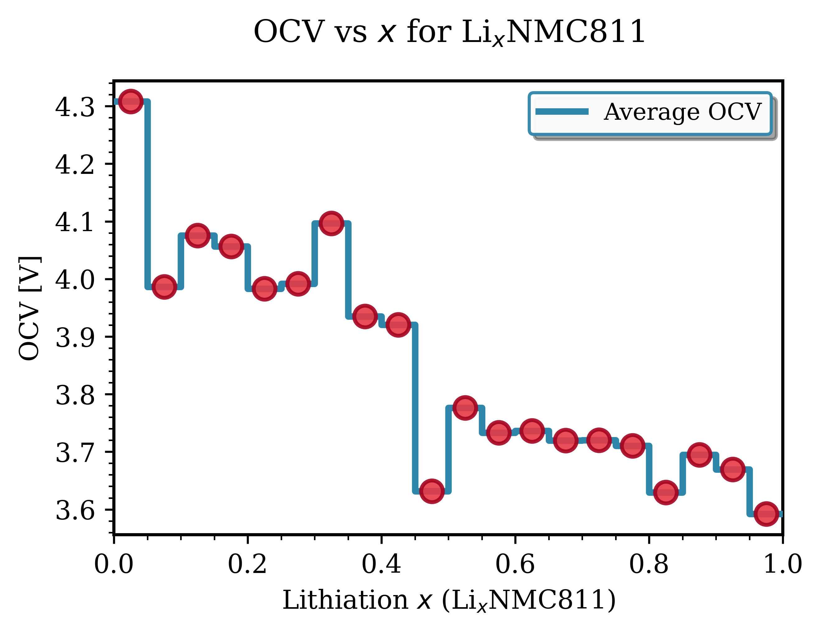
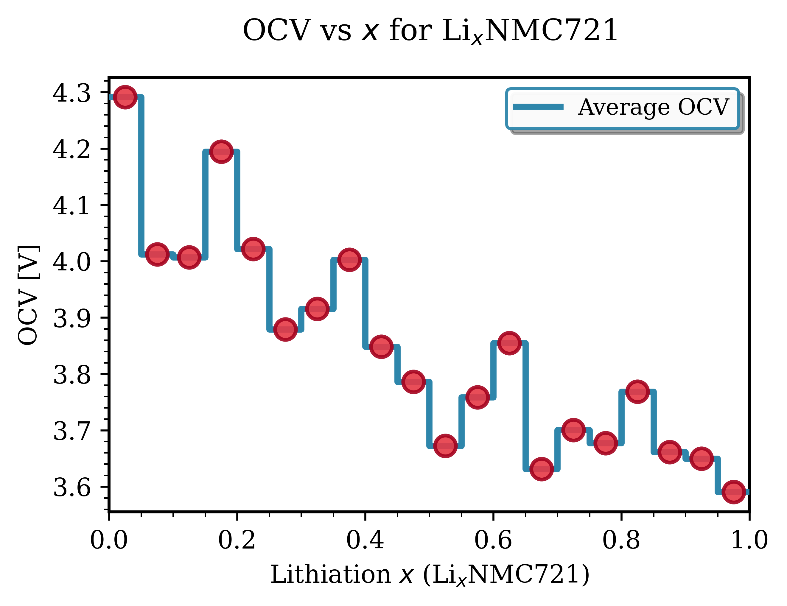
Fig. 140 LixNMC811 (Ni₀.₈Mn₀.₁Co₀.₁O₂)	Fig. 141 LixNMC721 (Ni₀.₇Mn₀.₂Co₀.₁O₂)
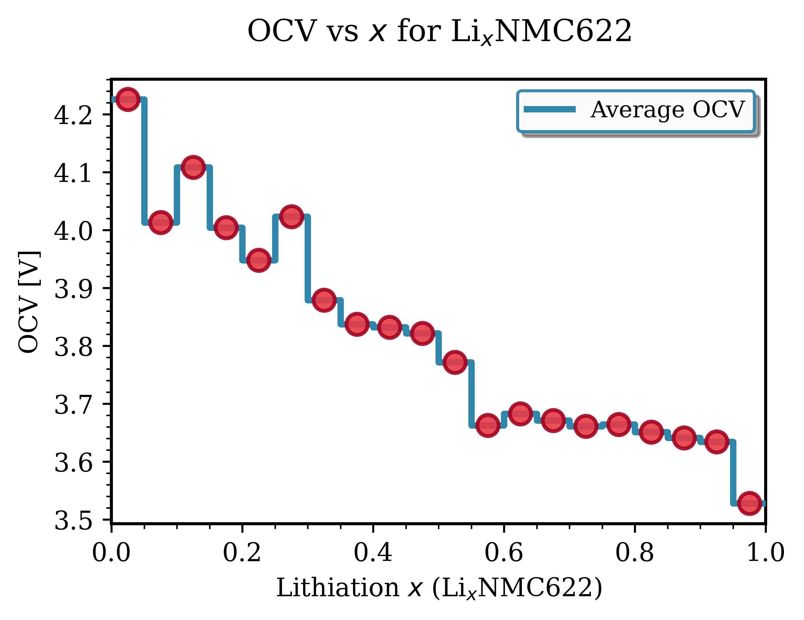
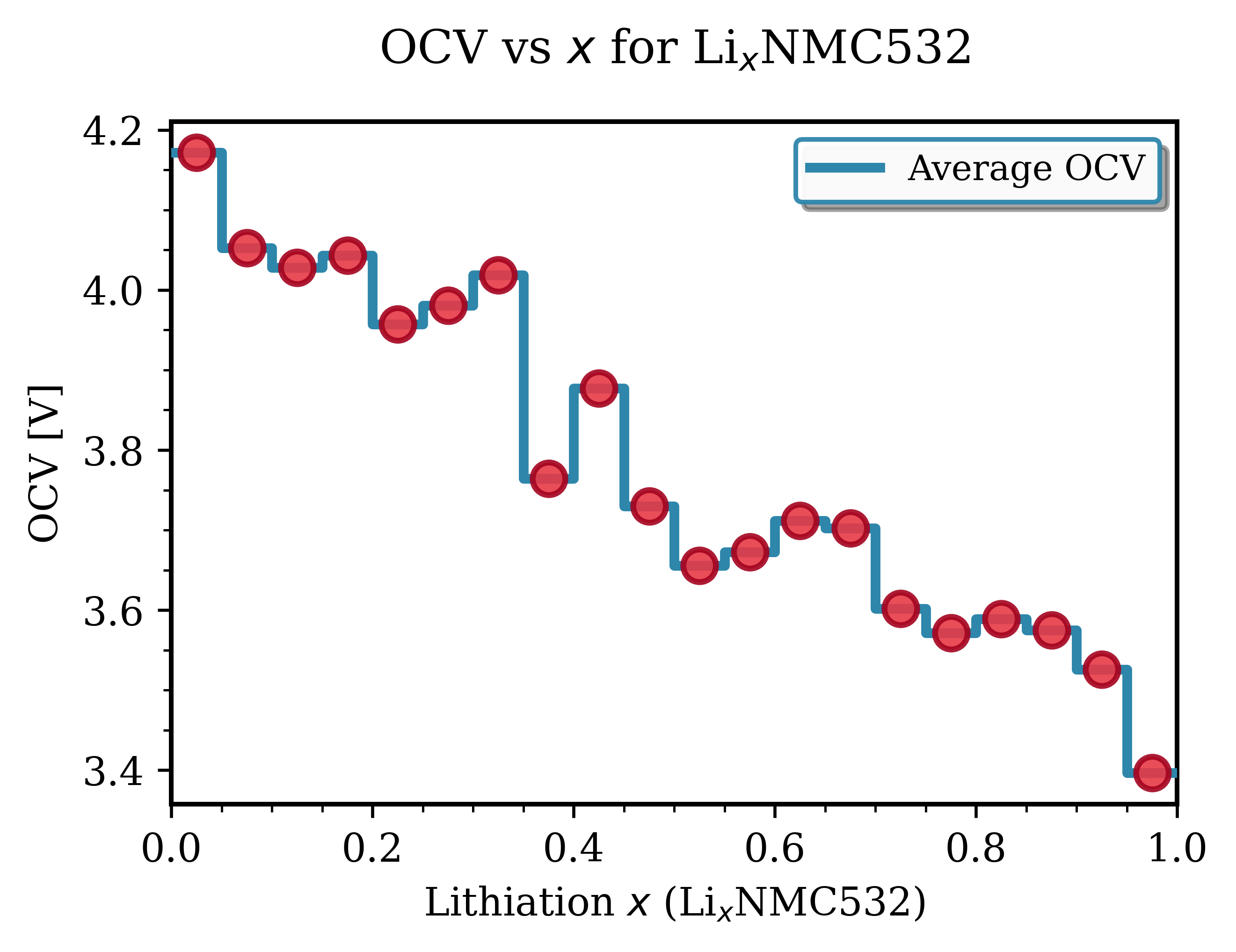
Fig. 142 LixNMC622 (Ni₀.₆Mn₀.₂Co₀.₂O₂)	Fig. 143 LixNMC532 (Ni₀.₅Mn₀.₃Co₀.₂O₂)

Key Observations for NMC Materials:

• Voltage range: Typically 3.6-4.3 V vs Li/Li⁺. Good agreement with experimental data [1].

• Smooth profiles: NMC exhibits continous, downward-sloping trend with increasing lithiation, characteristic of solid-solution behavior.

OCV Curve for LiFePO₄

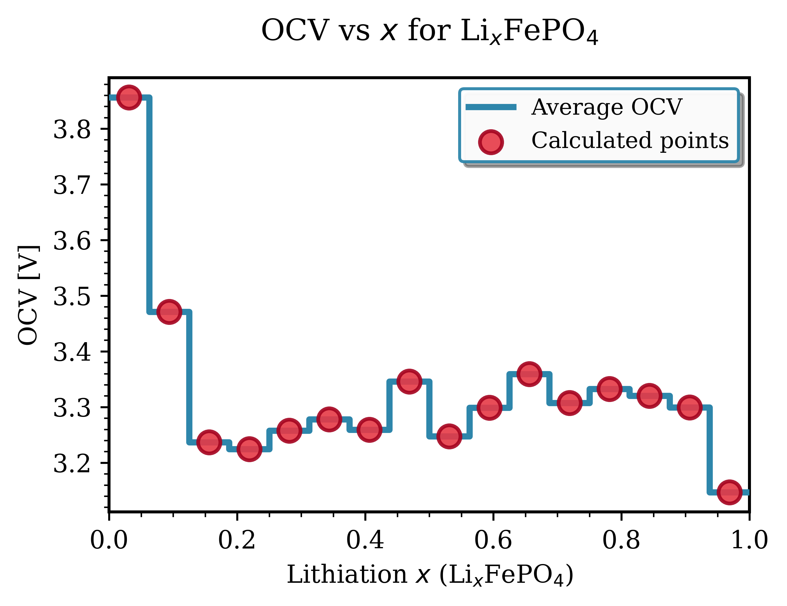
Fig. 144 OCV curve for Li_xFePO₄. The flat plateau at ~3.3 V indicates two-phase coexistence between lithiated (LiFePO₄) and delithiated (FePO₄) phases.

Key Observations for LiFePO₄:

• Voltage range: 3.6-4.3 V, dominated by a flat plateau at ~3.3 V vs Li/Li⁺. Good agreement with experimental OCV measurements [2][3].

• Two-phase region: The flat plateau is a signature of a two-phase coexistence region (phase separation).

Computational Performance

With MatterSim MLFF (default):

• Total calculation for NMC: ~3-5 hours for 21 compositions × 150 samples = 3,150 relaxations (1 process, 30 threads, 1 GPU: NVIDIA A100-SXM4-80GB)

• Total calculation for LFP: ~2-3 hours for 17 compositions × 150 samples = 2,550 relaxations (similar hardware)

Running the Scripts

Using the Jobs tool (recommended for long calculations):

Submit as a batch job in NanoLab:

1. Open Jobs tool → Click Add new job

2. Navigate to your working directory and select the OCV script:

   • For NMC: ocv_vs_lithiation_NMC.py

   • For LFP: ocv_vs_lithiation_LFP.py

   • Click Open

3. In the Jobs setting tab:

   • Set Number of processes: 8-16 (for MLFF) or 32-64 (for DFT, GPUs recommended)

   • Adjust memory and time limits as needed

4. In the Files I/O tab, add required input files:

   • For LFP: Add DFTcalculator.py and configuration.py

   • For NMC: No additional files needed (only the SQS structure already in the script)

5. Click Submit to queue

Output Files

From config_NMC.py (SQS generation, NMC only):

• LiCoO2_template.hdf5: R-3m LiCoO₂ primitive cell template

• NMC_binary_Ni_Zn_SQS.hdf5: Binary SQS (Ni vs Zn placeholder, intermediate)

• NMC{comp_tag}_SQS_final.hdf5: NMC structure after Zn→Mn+Co split (unoptimized)

• NMC{comp_tag}_SQS_final_optimized.hdf5: Relaxed SQS structure - use as input for OCV

where {comp_tag} is formed from the composition fractions: e.g., NMC with Ni=0.8, Mn=0.1, Co=0.1 → 811; Ni=0.6, Mn=0.2, Co=0.2 → 622

From ocv_vs_lithiation_NMC.py:

• ocv_{NMC_TAG}_all.hdf5: All configurations and energies (for post-analysis)

• ocv_{NMC_TAG}_best.hdf5: Ground state structures (for structural analysis)

• ocv_{NMC_TAG}.png: Voltage curve plot (600 dpi)

• ocv_{NMC_TAG}.log: Calculation log

From ocv_vs_lithiation_LFP.py:

• ocv_LiFePO4_all.hdf5: All optimized structures and energies

• ocv_vs_x.png: Voltage curve plot (600 dpi)

• ocv_vs_x.txt: Tab-separated voltage data

• ocv_LFP.log: Calculation log

Advanced Extensions

Entropy Corrections for Finite Temperature

For more realistic finite-temperature OCV, apply Nernstian entropy correction for solid-solution materials (NMC only, not LFP). The method loads ground-state voltages from standard OCV calculation (0 K energies), calculates the Nernstian entropy term \(\Delta V = (k_B \cdot T) \times \ln((1-x)/x)\) for each composition point, and adds it to the 0 K voltage. The approach assumes random Li/vacancy mixing (ideal solution approximation) with configurational entropy \(S = -k_B[x \cdot \ln(x) + (1-x) \cdot \ln(1-x)]\) and no Li-Li interaction energy. The entropy correction smooths the voltage curve and shifts voltages but is valid only for solid solutions (NMC), not two-phase materials (LFP). See ocv_vs_lithiation_nmc_config_entropy.py for implementation.

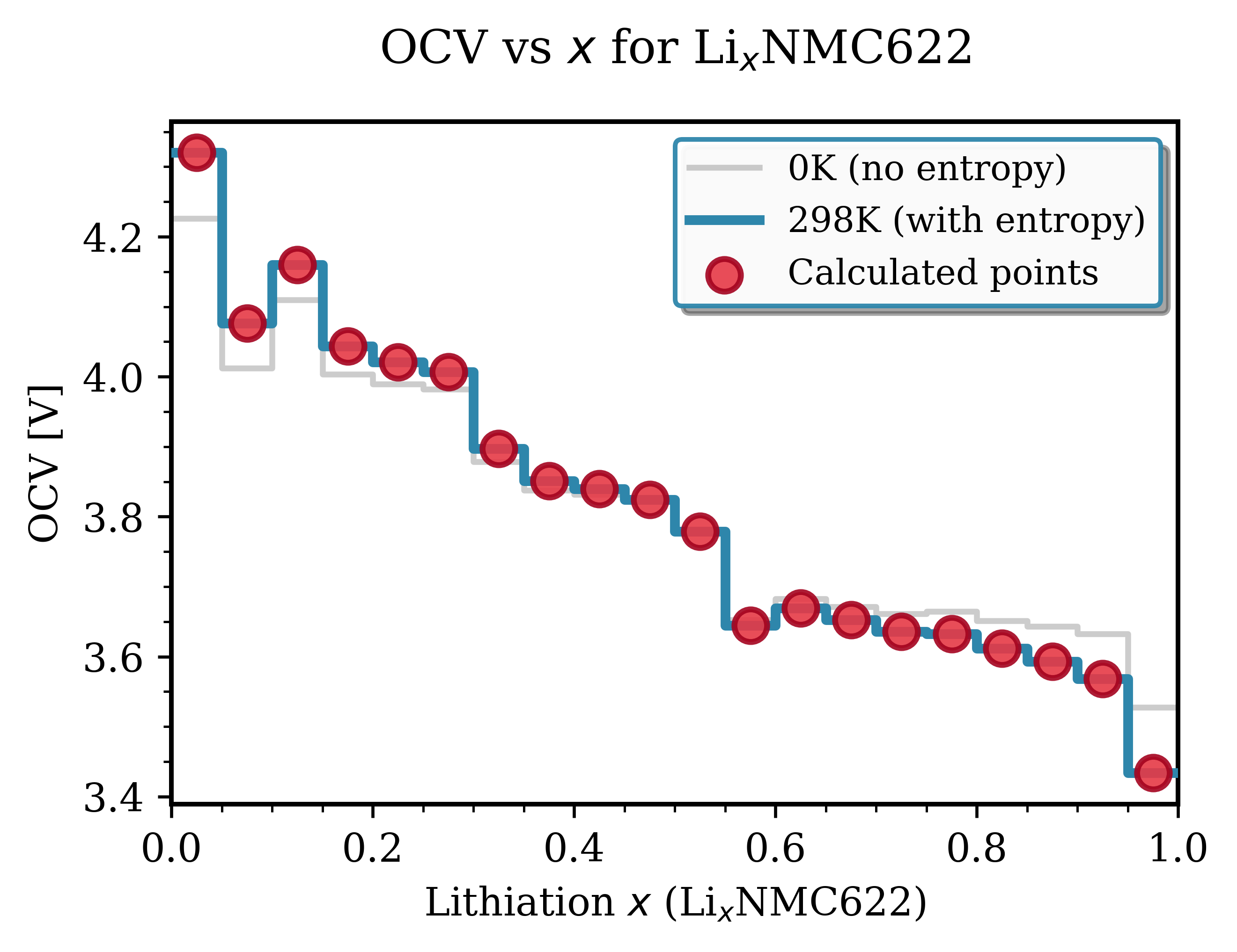
Fig. 145 Entropy-corrected OCV for NMC622. Comparison of 0 K voltage (gray, from ground-state energies only) and 298 K voltage (blue, including configurational entropy correction). The entropy term smooths the curve and shifts voltages.

Structural Analysis

Analyze volume and c-axis changes during (de)lithiation from ground state structures in ocv_*_best.hdf5. The method loads ground-state configurations, extracts lattice vectors for each lithiation level, calculates volume and c-axis length, and normalizes to the fully lithiated state (x = 1.0) to obtain relative changes ΔV/V₀ and Δc/c₀. The c-axis and volume contract significantly at deep delithiation (x < 0.2), particularly pronounced in Ni-rich compositions (NMC811), correlating with cycling-induced mechanical stress and capacity fade. See volume_caxis_vs_lithiation.py for implementation.

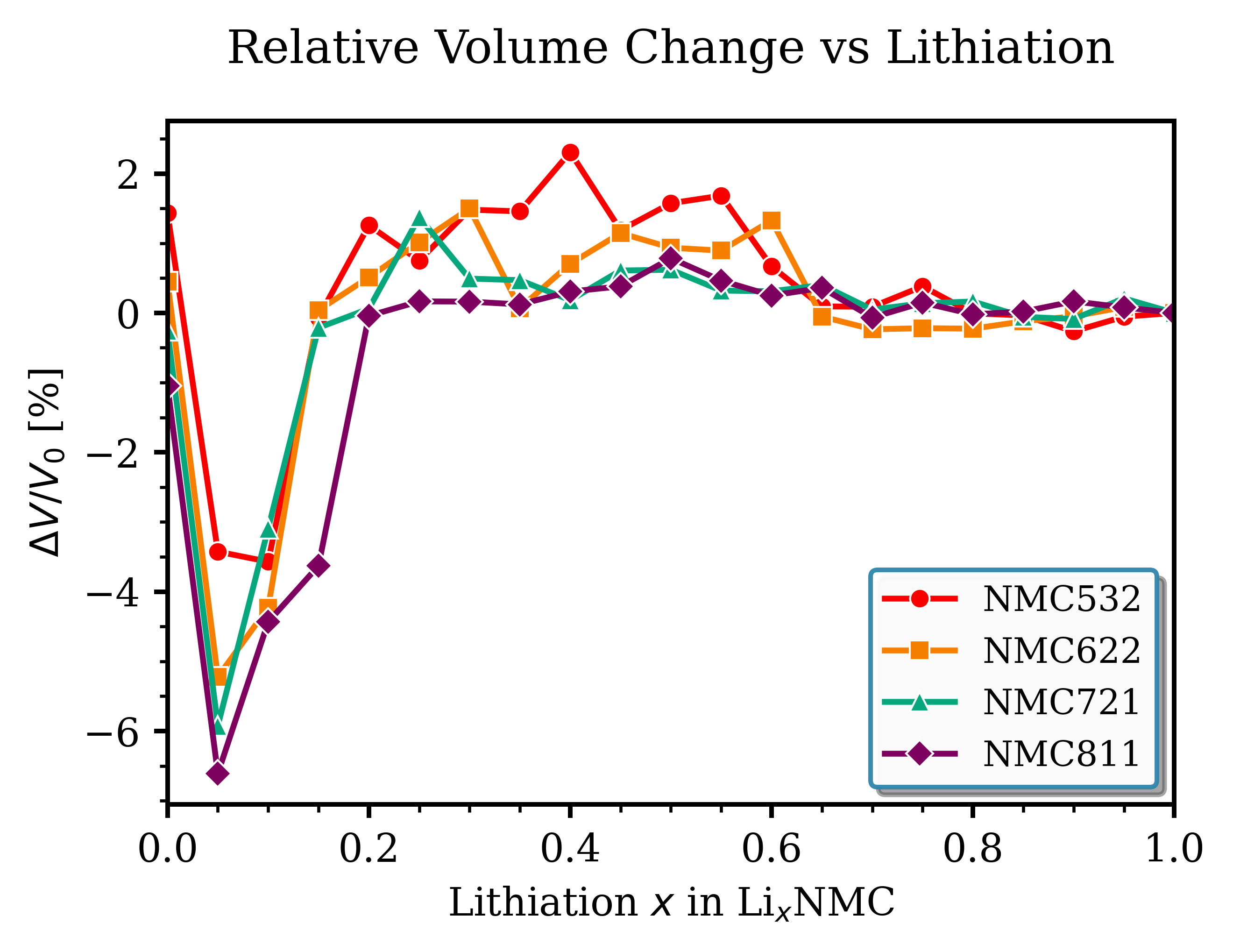
Fig. 146 Relative volume change vs. lithiation. Volume contraction upon delithiation is most pronounced in Ni-rich NMC.

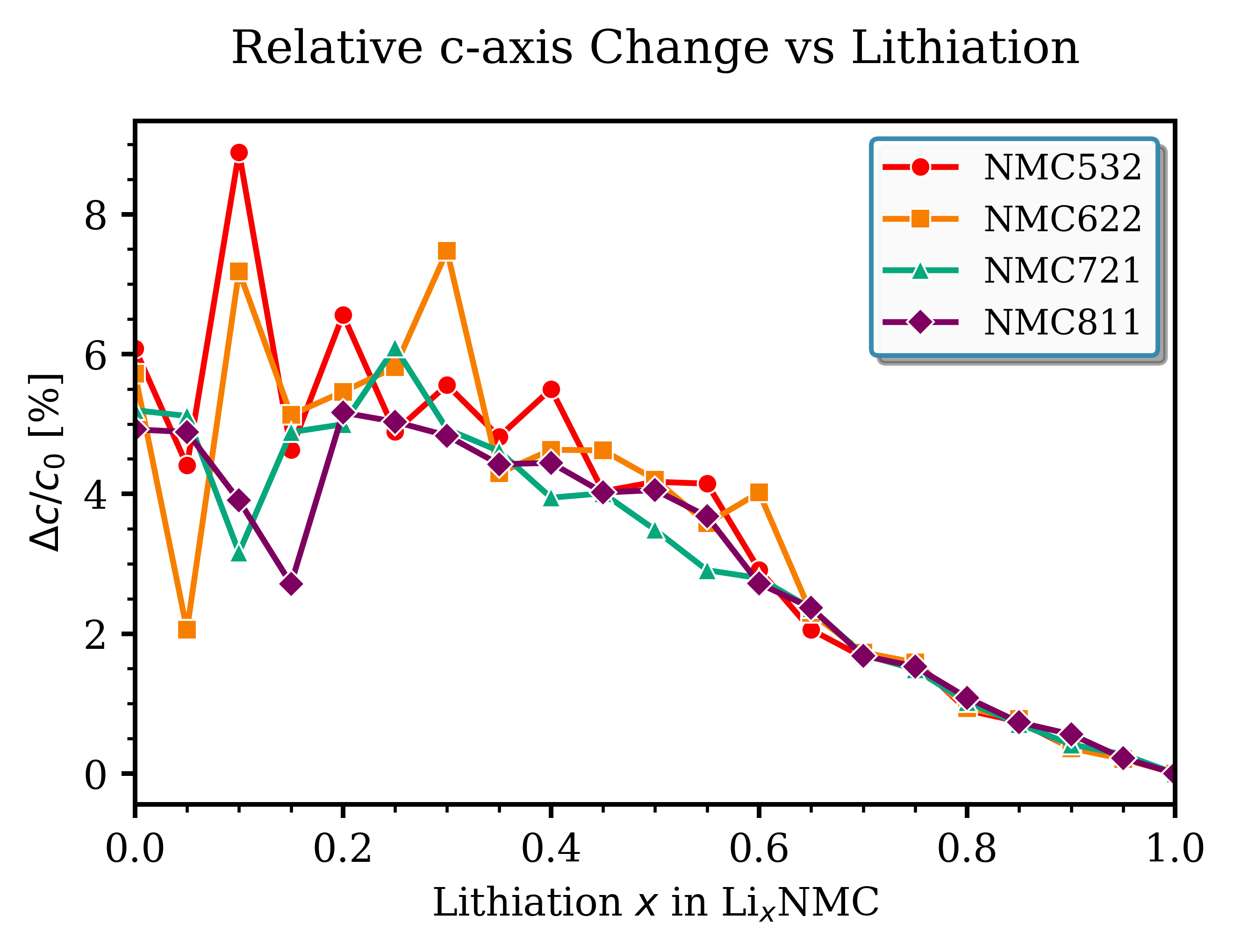
Fig. 147 Relative c-axis change vs. lithiation. The c-axis contracts more than a/b axes due to TM-O layer compression.

Summary

This application provides a complete workflow for predicting battery OCV curves from first-principles atomistic simulations. The workflow handles both layered NMC (with SQS disorder modeling) and olivine LFP cathodes, uses intelligent configurational sampling to find ground states at each lithiation level, and supports both fast MLFF and accurate DFT calculations. The methodology enables rapid screening of cathode chemistries and can be extended to new materials (LNMO, Li-rich oxides), doping studies and finite-temperature corrections.

References

[1] (1,2)

Hyung-Joo Noh, Sungjune Youn, Chong Seung Yoon, and Yang-Kook Sun. Comparison of the structural and electrochemical properties of layered li [nixcoymnz] o2 (x= 1/3, 0.5, 0.6, 0.7, 0.8 and 0.85) cathode material for lithium-ion batteries. Journal of power sources, 233:121–130, 2013. URL: https://www.sciencedirect.com/science/article/abs/pii/S0378775313001110, doi:https://doi.org/10.1016/j.jpowsour.2013.01.063.

[2] (1,2)

Amardeep Sidhu, Afshin Izadian, and Sohel Anwar. Adaptive nonlinear model-based fault diagnosis of li-ion batteries. IEEE Transactions on Industrial Electronics, 62(2):1002–1011, 2014. URL: https://ieeexplore.ieee.org/abstract/document/6851886, doi:10.1109/TIE.2014.2336599.

[3] (1,2)

Federico Baronti, Walter Zamboni, Roberto Roncella, Roberto Saletti, and Giovanni Spagnuolo. Open-circuit voltage measurement of lithium-iron-phosphate batteries. In 2015 IEEE International Instrumentation and Measurement Technology Conference (I2MTC) Proceedings, 1711–1716. ieee, 2015. URL: https://ieeexplore.ieee.org/abstract/document/7151538, doi:10.1109/I2MTC.2015.7151538.