Surface Phase Diagram Construction

This application demonstrates how to construct surface phase diagrams for catalytic and reactive surfaces as functions of temperature and gas-phase chemical potentials. Phase diagrams are essential tools for understanding surface stability and reactivity under realistic environmental conditions in heterogeneous catalysis, electrochemistry, and materials science.

Important

QuantumATK Version: This application is designed for QuantumATK X-2025.06.

Module Requirement: This application requires the SurfacePhaseDiagram module for surface phase diagram generation. The module is provided as a compiled Python file (.pye) and must be available in your Python path. You can download it from the attached files.

This application uses thermochemistry data from DFT calculations to construct phase diagrams. You can download the required files below:

• SurfacePhaseDiagram.pye - Compiled Python module (Essential - must be in the path)

• SurfacePhaseDiagram2D.py - Example script for RuO₂-H₂O-O₂ system

• SurfacePhaseDiagram2D.hdf5 - Workflow for 2D phase diagram generation

• thermochemistry_database.zip - Thermochemistry database

Key Features

• Chemical potential representation: Maps stable surface phases as functions of gas-phase chemical potentials

• Temperature-pressure diagrams: Alternative representation showing phase stability vs. temperature and pressure

• Multi-species support: Handles binary gas environments (e.g., H₂O and O₂, CO and O₂)

• Multiple phases: Determines most stable configuration among clean and various adsorbate-covered surfaces

• Flux calculations: Provides molecular flux information for experimental comparison

• Customizable plots: Generates high-quality phase diagrams

Scientific Background

Surface Phase Diagrams in Catalysis

Surface phase diagrams provide crucial insights into:

• Catalyst active phases: Which surface termination is stable under reaction conditions

• Reaction mechanisms: How surface composition changes affect catalytic activity

• Poisoning and deactivation: Understanding conditions where unwanted species dominate

• Operando conditions: Relating in-situ observations to surface structures

Theoretical Framework

The phase diagram is constructed by calculating the surface free energy (γ) as a function of chemical potentials (μ) for each gas-phase species:

\[\gamma(T, \mu_{\text{O}_2}, \mu_{\text{H}_2\text{O}}) = \frac{1}{2A} \left[ G_{\text{surf}}(T) - n_{\text{bulk}} G_{\text{bulk}}(T) - n_{\text{O}_2} \mu_{\text{O}_2}(T,p) - n_{\text{H}_2\text{O}} \mu_{\text{H}_2\text{O}}(T,p) \right]\]

where:

• A is the surface area per unit cell

• G_surf is the Gibbs free energy of the surface configuration

• G_bulk is the Gibbs free energy per formula unit of bulk material

• n_bulk is the number of bulk formula units in the surface slab

• n_species are the numbers of adsorbed molecules

• μ_species are the chemical potentials of gas-phase species

The chemical potential relates to pressure through:

\[\mu(T,p) = \mu^0(T,p_0) + k_B T \ln\left(\frac{p}{p_0}\right)\]

At each point in (μ₁, μ₂) space, the phase with the lowest surface free energy is thermodynamically stable.

Example System: RuO₂ in H₂O/O₂ Environment

The example system demonstrates phase diagram construction for RuO₂(110), a model oxide catalyst, in contact with water vapor and oxygen gas. This system is relevant for:

• Surface is in equilibrium with humid environments

• Multiple gaseous species influence surface stability

Surface Configurations

The phase diagram includes multiple competing surface terminations:

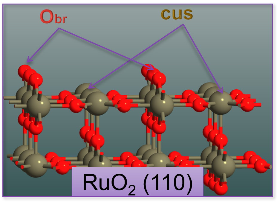
Fig. 150 RuO₂(110) surface structure showing key adsorption sites. The surface features coordinatively unsaturated Ru atoms (cus sites) and bridge oxygen atoms (br sites) that serve as active sites for molecular and dissociative water adsorption.

1. Clean Surface (O_br/-)

The bare RuO₂(110) surface with coordinatively unsaturated Ru and bridge oxygen sites

2. Molecular Water Adsorption (H₂O/cus)

Water molecules physisorbed on coordinatively unsaturated (cus) Ru sites

3. Dissociated Water (2OH/cus+br)

Water dissociated into OH groups on both cus and bridge (br) sites

4. Hydroxylated + Water (OH + H₂O)

Mixed phase with both OH groups and molecular water

5. Oxygen Terminations (O/cus, 2O)

Additional oxygen atoms adsorbed on the surface from O₂ dissociation

Workflow Overview

The complete workflow consists of six main steps:

STEP 1: Generate Surface Configurations
        ↓
STEP 2: Calculate DFT Energies & Thermochemistry
        ↓
STEP 3: Store Thermochemistry in Database
        ↓
STEP 4: Define System Parameters
        ↓
STEP 5: Configure Phase Diagram Script
        ↓
STEP 6: Generate Phase Diagram

STEP 1: Generate Surface Configurations

Use QuantumATK’s Builder tools to create all relevant surface structures:

1. Create clean surface:

   • Use Surface (Cleave) tool to generate the desired surface orientation

   • Optimize slab thickness (typically 3-5 atomic layers plus vacuum)

   • Add appropriate vacuum spacing (>10 Å)

2. Generate adsorbate configurations:

   • Open the Adsorption Tool (Builder → Surface Tools → Add Adsorbates)

   • Add water molecules at different sites (atop, bridge, hollow)

   • Create dissociated configurations (OH, O species)

   • Consider different coverages (1/2, 1/4, full monolayer)

3. Save all configurations as separate structure files for subsequent calculations

Tip

For systematic exploration, generate a comprehensive set of possible adsorption configurations. The phase diagram will automatically identify which are stable under different conditions.

STEP 2: Calculate Thermochemistry Properties

Compute thermochemistry data for all species using appropriate workflow templates:

For Gas-Phase Species (H₂O, O₂):

# Use IdealGasThermoChemistry workflow
# This calculates:
#   - Optimized geometry
#   - Electronic energy
#   - Vibrational frequencies
#   - Rotational and translational contributions
#   - Temperature-dependent free energy

For Bulk and Surface Configurations:

# Use CrystalThermoChemistry workflow
# This calculates:
#   - Optimized crystal structure
#   - Electronic energy
#   - Phonon density of states (optional for T > 0)
#   - Temperature-dependent free energy

Note

Computational settings recommendations:

• Use consistent DFT functional for all calculations (e.g., PBE)

• Converge k-point sampling and basis set cutoffs

• For surfaces: Use sufficient slab thickness and vacuum

• Include spin polarization where relevant (O₂, transition metal oxides)

STEP 3: Upload Thermochemistry to Database

Store computed thermochemistry data in QuantumATK’s thermochemistry database:

1. Access the database:

   • Open Thermochemistry Analyzer in NanoLab

   • Click Database button to open database window

   • Default location: C:\Users\username\.quantumatk\databases\thermochemistry\

2. Create entries:

   • Click Add Entry for each calculated configuration

   • Provide unique, descriptive names (e.g., “RuO2_bulkDFT”, “RuO2_OH_cusDFT”)

   • Upload the corresponding thermochemistry object from your calculation files

3. Organize entries:

   • Use systematic naming conventions

   • Document stoichiometry and configuration details

   • Keep track of all entry names for the script configuration

4. Alternatively:

   • Open the database folder (default location: C:\Users\username\.quantumatk\databases\thermochemistry\)

   • Copy the thermochemistry objects directly into the folder with unique names

   • Note: No multipliers will be set when using this method

STEP 4: Define System Parameters

Set the physical parameters for your phase diagram at the top of the script:

# Temperature and pressure reference
temperature = 100.0 * Kelvin        # Operating temperature
p0 = 1.013 * bar                    # Reference pressure (1 atm)

# Chemical potential ranges for species 1 (e.g., H₂O)
mu_species1_min = -2.5 * eV
mu_species1_max = 0.5 * eV

# Chemical potential ranges for species 2 (e.g., O₂)
mu_species2_min = -2.5 * eV
mu_species2_max = 0.0 * eV

# Molecular masses for flux calculations
mass_species1 = 18.015 * atomicMassUnit  # H₂O
mass_species2 = 32.0 * atomicMassUnit    # O₂

Tip

Choosing chemical potential ranges:

• Typical range: -3 to 0 eV relative to gas-phase reference

• Lower μ: low pressure/activity conditions

• Higher μ: high pressure/activity conditions

• Adjust based on relevant experimental conditions

STEP 5: Configure Script Parameters

Edit the script to match your system by updating three main configuration dictionaries:

A. SYSTEM_ENTRIES Dictionary

Define all database entry names and stoichiometry:

SYSTEM_ENTRIES = {
    # Bulk reference
    'bulk_config': 'RuO2_bulkDFT',           # Database entry name
    'bulk_stoichiometry': 2.0,                # Formula units in bulk

    # Gas phase references
    'gas_species2': 'O2DFT',                  # O₂ gas thermochemistry
    'gas_species1': 'H2ODFT',                 # H₂O gas thermochemistry

    # Clean surface
    'clean_surface': 'RuO2_O_brDFT',          # Clean surface entry
    'surface_stoichiometry': 8.0,             # Bulk units in slab
    'clean_surface_label': 'Obr/-',           # Plot label

    # Adsorbate configurations
    'surf_ad_configs': [
        {
            'name': 'RuO2_OH2_cusDFT',        # Database entry
            'label': 'H\ :sub:`2`\ O/cus',    # Plot label
            'color': 'skyblue',                # Phase color
            'n_species1': 1.0,                 # Number of H₂O
            'n_species2': 0.0,                 # Additional O atoms
        },
        {
            'name': 'RuO2_2OH_cus_brDFT',
            'label': '2OH/cus+br',
            'color': 'lightgreen',
            'n_species1': 1.0,                 # From dissociated H₂O
            'n_species2': 0.0,
        },
        # Add more configurations...
    ],
}

B. PHASE_DIAGRAM_CONFIG Dictionary

Set the phase diagram grid and display parameters:

PHASE_DIAGRAM_CONFIG = {
    # Chemical potential grid
    'del_mu_species2_range': (
        mu_species2_min.inUnitsOf(eV),
        mu_species2_max.inUnitsOf(eV),
        0.01,  # Step size in eV
    ),
    'del_mu_species1_range': (
        mu_species1_min.inUnitsOf(eV),
        mu_species1_max.inUnitsOf(eV),
        0.01,
    ),

    # Pressure axis tick positions
    'pressure_ticks_species2': (
        mu_species2_min.inUnitsOf(eV),
        mu_species2_max.inUnitsOf(eV),
        0.5,  # Tick spacing
    ),
    'pressure_ticks_species1': (
        mu_species1_min.inUnitsOf(eV),
        mu_species1_max.inUnitsOf(eV),
        0.5,
    ),

    'reference_pressure': p0,
    'title': 'RuO\ :sub:`2`\ (110) Surface Phase Diagram',
    'output_filename': 'surface_phase_diagram.png',
}

C. PLOT_CONFIG Dictionary

Customize plot appearance:

PLOT_CONFIG = {
    'figure_size': (18, 16),           # Width, height in inches
    'dpi': 300,                         # Resolution
    'title_fontsize': 16,
    'label_fontsize': 16,
    'tick_fontsize': 14,
    'phase_label_fontsize': 12,
    'clean_surface_color': 'violet',   # Color for clean surface
}

STEP 6: Run the Phase Diagram Script

Execute the script to generate the phase diagram:

# Import the module
import SurfacePhaseDiagram as surface_phase_diagram

# Generate the plot
fig, stable_phase_index, thermo_data = surface_phase_diagram.generate_surface_phase_diagram(
    SYSTEM_ENTRIES,
    PHASE_DIAGRAM_CONFIG,
    PLOT_CONFIG,
    MOLECULAR_MASSES,
    temperature,
    p0,
)

The script will:

1. Load all thermochemistry data from the database

2. Create a 2D grid in (μ₁, μ₂) space

3. Calculate surface free energy for each phase at each grid point

4. Determine the most stable phase at each point

5. Generate a color-coded phase diagram with multiple axes

6. Save the plot as a high-resolution PNG file

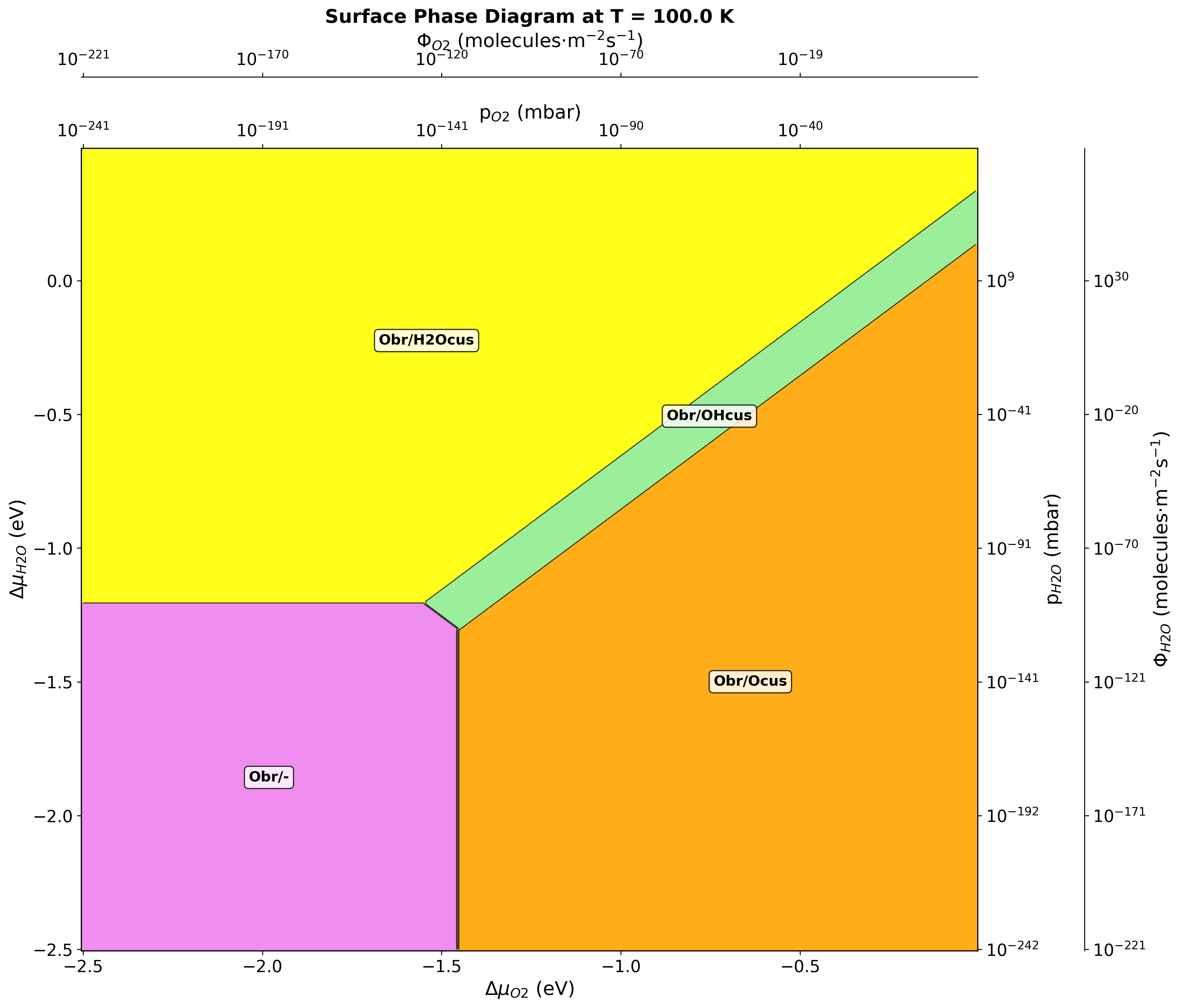
Fig. 151 Surface phase diagram for RuO₂(110) in H₂O-O₂ environment at 100 K. Different colors represent stable phases: clean surface (violet), molecular water adsorption (yellow), dissociated water (green), and oxygen-rich terminations (red/orange).

Temperature-Pressure Phase Diagrams

Alternative Representation

Instead of chemical potentials, phase diagrams can be plotted as temperature vs. pressure:

# Generate T-P diagram instead of μ₁-μ₂ diagram
fig, stable_phase_index, thermo_data = surface_phase_diagram.generate_temperature_pressure_diagram(
    SYSTEM_ENTRIES,
    TEMP_PRESSURE_CONFIG,
    PLOT_CONFIG,
)

Configuration for T-P diagrams:

TEMP_PRESSURE_CONFIG = {
    'temperature_range': (100, 1000, 10),   # Min, max, step in K
    'pressure_range': (1e-10, 1e5, 100),    # Min, max, steps in bar
    'fixed_gas_species': 'gas_species1',     # Which gas to vary
    'fixed_gas_pressure': 1e-3 * bar,        # Pressure of fixed gas
    'output_filename': 'phase_diagram_TP.png',
}

This representation is more intuitive for experimental comparison and directly shows operating windows for catalytic processes.

Advanced Usage

Multiple Temperature Comparison

Generate phase diagrams at different temperatures to understand temperature effects:

temperatures = [100, 300, 500, 800] * Kelvin

for T in temperatures:
    fig, _, _ = surface_phase_diagram.generate_surface_phase_diagram(
        SYSTEM_ENTRIES,
        PHASE_DIAGRAM_CONFIG,
        PLOT_CONFIG,
        MOLECULAR_MASSES,
        temperature=T,
        p0=p0,
    )
    # Save with temperature-specific filename

Running the Script

The complete script can be executed in several ways:

From NanoLab:

1. Open the script file in the Scripteditor

2. Click Send To → Job Manager

3. Or select the file and use Jobs tool to execute

From Command Line:

atkpython SurfacePhaseDiagram2D.py

Note

Running the Script Locally

This script requires access to the thermochemistry database containing all computed thermochemistry objects for the bulk, gas-phase species, clean surface, and adsorbate configurations. The script must be executed locally on a system where:

• The thermochemistry database is available and properly configured

• All required thermochemistry entries have been calculated and uploaded to the database

• The SurfacePhaseDiagram.pye module is in the Python path

Output Files

The script generates:

• surface_phase_diagram.png: The complete phase diagram with all axes

• Console output: Progress information and verification messages

The phase diagram image includes:

• Color-coded phase regions

• Chemical potential axes (eV)

• Pressure scales (mbar)

• Molecular flux scales (molecules·m⁻²·s⁻¹)

• Phase labels

• Temperature and title information

Further Reading

Theoretical Background:

• Reuter, K., & Scheffler, M. (2001). “Composition, structure, and stability of RuO₂(110) as a function of oxygen pressure.” Physical Review B, 65(3), 035406.

• Reuter, K., & Scheffler, M. (2003). “Composition and structure of the RuO₂(110) surface in an O₂ and CO environment: Implications for the catalytic formation of CO₂.” Physical Review B, 68(4), 045407.

• Knapp, M., Crihan, D., Seitsonen, A. P., Lundgren, E., Resta, A., Andersen, J. N., & Over, H. (2006). “Effect of a humid environment on the surface structure of RuO₂(110).” Journal of Physical Chemistry B, 110(30), 14007-14010.

Summary

This application enables construction of surface phase diagrams from first-principles thermochemistry calculations. Key capabilities include:

✓ Map stable surface phases as functions of gas-phase chemical potentials or T-P conditions

✓ Support for multi-species environments and complex surface configurations

✓ Flexible framework adaptable to different material systems and conditions

Phase diagrams provide essential insights for understanding and predicting surface behavior under realistic environmental conditions, bridging the gap between computational predictions and experimental observations in catalysis, electrochemistry, and materials science.