DensityPredictor
Included in QATK.Calculators.DFT, QATK.MLDFT
- class DensityPredictor(model=None, probe_count=None, gpu_acceleration=None, density_model=None)
Class for parameters needed for a density predictor.
- Parameters:
model (GridValuesModel) – Class specifying the path to the density model.
probe_count (int, optional) – Number of probe graph nodes to use, Default:
5000.gpu_acceleration (Enabled | Disabled | Automatic, optional) – Whether to use GPU acceleration. If set to
Automatic, the predictor will use the GPU if available. Default:Automatic
- densityModel()
Get the density model used by this predictor. Deprecated, use model() instead.
- Returns:
The density model.
- Return type:
- gpuAcceleration()
Return whether to use CUDA-supported GPU acceleration.
- Returns:
The GPU acceleration flag.
- Return type:
Enabled | Disabled | Automatic
- model()
Return the parameters for the ml model.
- Returns:
The model parameters.
- Return type:
- nlinfo()
- Returns:
The nlinfo.
- Return type:
dict
- predictElectronDensity(configuration, calculator, ground=None)
Use the defined model to predict the electron density of a configuration.
- Parameters:
configuration (MoleculeConfiguration | BulkConfiguration | DeviceConfiguration) – The configuration for which to predict the electron density.
calculator (Calculator) – The calculator used to predict the electron density.
ground (bool) – Boolean controlling if the average electron difference density should be forced to zero.
- Returns:
The predicted electron density.
- Return type:
NLEngine.MPISharedScalarField
- predictElectronDifferenceDensity(configuration, calculator, ground=None)
Use the defined model to predict the electron difference density of a configuration.
- Parameters:
configuration (MoleculeConfiguration | BulkConfiguration | DeviceConfiguration) – The configuration for which to predict the electron density.
calculator (Calculator) – The calculator used to predict the electron density.
ground (bool) – Boolean controlling if the average electron difference density should be forced to zero.
- Returns:
The predicted electron density.
- Return type:
NLEngine.MPISharedScalarField
- predictElectronDifferenceDensityFromModel(deep_dft_model, configuration, calculator, ground=None)
Use the given model to predict the electron difference density of a configuration.
- Parameters:
deep_dft_model (DeepDFTModel) – The deep DFT model to use for the prediction.
configuration (MoleculeConfiguration | BulkConfiguration | DeviceConfiguration) – The configuration for which to predict the electron density.
calculator (Calculator) – The calculator used to predict the electron density.
ground (bool) – Boolean controlling if the average electron difference density should be forced to zero. Default:
True
- Returns:
The predicted electron density.
- Return type:
NLEngine.MPISharedScalarField
- probeCount()
Return the number of probes to use for the grid prediction.
- Returns:
The number of probes.
- Return type:
int
- uniqueString()
Return a unique string representing the state of the object.
Notes
Using a machine learned density predictor can significantly speed up the convergence of the self-consistent field (SCF) procedure in density functional theory (DFT) calculations. The predictor provides an initial guess for the electron density, which can reduce the number of iterations required to reach convergence.
The way to use a density predictor in a DFT calculation is to create an instance of the DensityPredictor class and pass it to the AlgorithmParameters used in the DFT calculation. For example,
model = PretrainedGridValuesModels.density_MP_PBE_PD_High_Y2026

grid_values_predictor = DensityPredictor(
  model=model,
)

algorithm_parameters = AlgorithmParameters(grid_values_predictor=grid_values_predictor)
where PretrainedGridValuesModels.density_MP_PBE_PD_High_Y2026 is a pre-trained density model included in QuantumATK.
Application of a density predictor is supported for both CPU-and GPU-based DFT calculations in QuantumATK. However, note that running on a GPU is significantly faster.
Use of a density predictor is supported for both LCAO and Plane Wave DFT calculations in QuantumATK, but currently only for normconserving pseudopotentials.
MGGA functionals cannot be used together with the density predictor. Other XC funcitonals are supported, but we recommend using the same XC functional as used during training of the density model for best results.
Pretrained models
QuantumATK includes a few pre-trained density models that can be used directly in DFT calculations. The pre-trained density models available in QuantumATK are listed below:
- density_MP_PBE_PD_High_Y2026 (Y-2026)
Model name: PretrainedGridValuesModels.density_MP_PBE_PD_High_Y2026
Description: General model trained on >93,000 configurations from the Materials Project (MP) database. Recommended for faster convergence of SCF calculations, especially for bulk calculations with periodic boundary conditions. Covers most elements in the periodic table, except Lanthanides, Actinides, and noble gasses.
Pseudopotential: PseudoDojo
Basis set: High
Exchange correlation: PBE
Spin: Unpolarized, Polarized
- SiGe (Y-2026)
Model name: PretrainedGridValuesModels.density_SiGe
Description: Specific model trained for Si, Ge, and their alloys. The model can be used for bulk and confined systems (slabs, or nanowires). Good results can be obtained from non-selfconsistent calculations. Covers Si, Ge, and H for surface passivation.
Pseudopotential: PseudoDojo
Basis set: Medium
Exchange correlation: PBE
Spin: Unpolarized
- III-V (Y-2026)
Model name: PretrainedGridValuesModels.density_III_V
Description: Specific model trained for III-V compounds and their alloys. The model is trained on bulk configuration with periodic boundary conditions including configurations with displaced atoms obtained from Molecular Dynamics simulations. Good results can be obtained from non-selfconsistent calculations. Covers group III elements Al, In, Ga, and group V elements P, As, Sb.
Pseudopotential: PseudoDojo
Basis set: Medium
Exchange correlation: PBE
Spin: Unpolarized
Usage Examples
Use the pre-trained density_MP_PBE_PD_High_Y2026 model for the initial density in a DFT calculation. For this example the number of SCF steps is reduced from 15 to 7 by using the pre-trained density_MP_PBE_PD_High_Y2026 model as compared to the default neutral atom initial density.:
from QATK.Analysis import *
from QATK.Calculators.DFT import *
from QATK.Core import *

# %% CoSi2

# Set up lattice
lattice = FaceCenteredCubic(5.356*Angstrom)

# Define elements
elements = [Cobalt, Silicon, Silicon]

# Define coordinates
fractional_coordinates = [[ 0.  ,  0.  ,  0.  ],
                          [ 0.25,  0.25,  0.25],
                          [ 0.75,  0.75,  0.75]]

# Set up configuration
cosi2 = BulkConfiguration(
    bravais_lattice=lattice,
    elements=elements,
    fractional_coordinates=fractional_coordinates
    )


# %% Set LCAOCalculator

# %% LCAOCalculator

# ----------------------------------------
# Exchange-Correlation
# ----------------------------------------
exchange_correlation = SGGA.PBE

# ----------------------------------------
# Basis Set
# ----------------------------------------
basis_set = [
    BasisGGAPseudoDojo.Silicon_High,
    BasisGGAPseudoDojo.Cobalt_High,
]

k_point_sampling = KpointDensity(
    density_a=4.0 * Angstrom, density_b=4.0 * Angstrom, density_c=4.0 * Angstrom
)

numerical_accuracy_parameters = NumericalAccuracyParameters(
    k_point_sampling=k_point_sampling
)

model = PretrainedGridValuesModels.density_MP_PBE_PD_High_Y2026

grid_values_predictor = DensityPredictor(
    model=model,
)

algorithm_parameters = AlgorithmParameters(grid_values_predictor=grid_values_predictor)

calculator = LCAOCalculator(
    basis_set=basis_set,
    exchange_correlation=exchange_correlation,
    numerical_accuracy_parameters=numerical_accuracy_parameters,
    checkpoint_handler=NoCheckpointHandler,
    algorithm_parameters=algorithm_parameters,
)


# %% Set Calculator

cosi2.setCalculator(calculator)

cosi2.update()

nlsave('CoSi2_results.hdf5', cosi2)


# %% TotalEnergy

total_energy_1 = TotalEnergy(configuration=cosi2)
nlsave('CoSi2_results.hdf5', total_energy_1)
density_predictor_pretrained_model_example.py
For the specifically trained models, density_SiGe and density_III_V, good results can often be obtained even without performing self-consistent calculations, by using the predicted density directly in a non-self-consistent DFT calculation. An example of this is shown in the figure below showing the band structure of a SiGe nanowire calculated using the density_SiGe model with a non-self-consistent calculation (dashed red lines) and a self-consistent calculation (solid black lines).
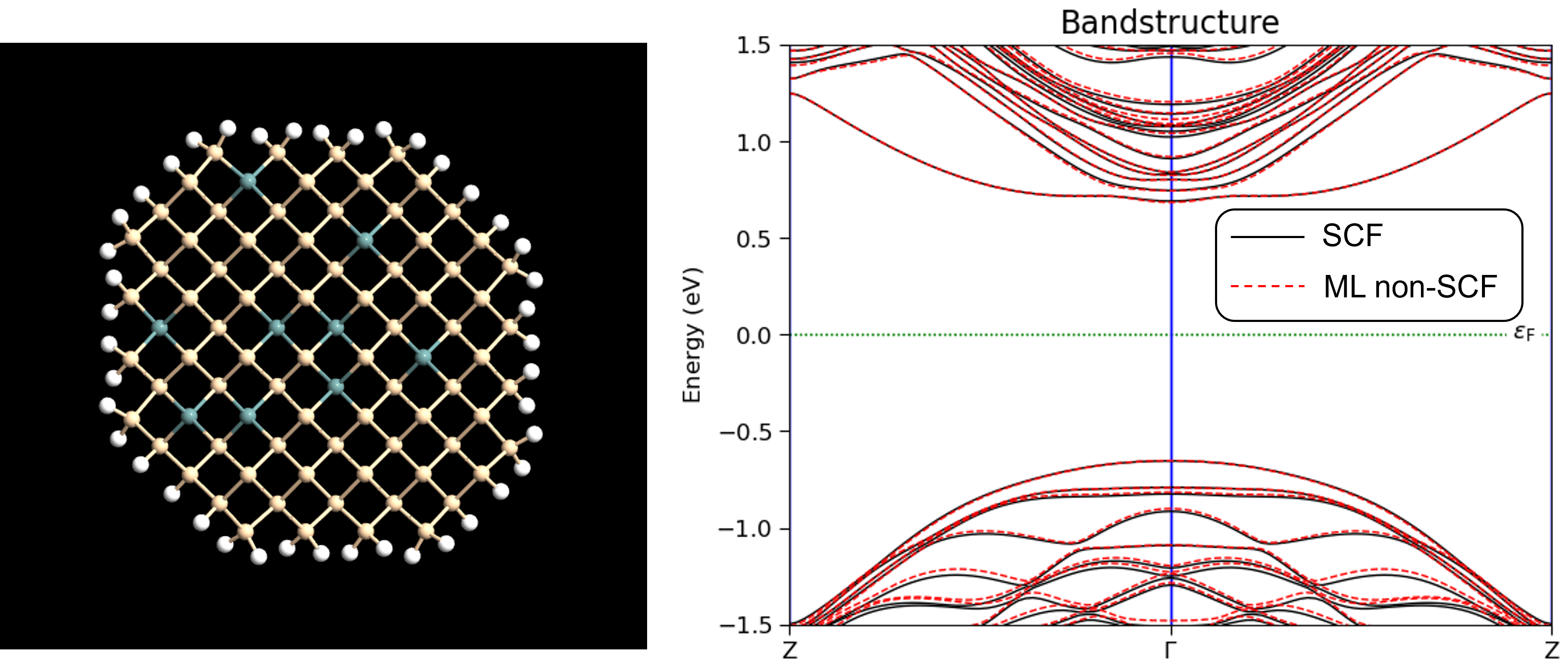
Illustration of SiGe nanowire configuration and bandstructure
The bandstructures were calculated with the following script: SiGe_nanowire.py .
Custom trained models
It is also possible to create custom GridValuesModels using the GridValuesModelTrainer class. In order to use a custom trained model with the DensityPredictor, one can load the model from the directory where it is stored as follows:
model = GridValuesModel(
    model_dir='/densitymodel/cutoff_4_model_3_128/'
)

grid_values_predictor = DensityPredictor(
    model=model,
)

algorithm_parameters = AlgorithmParameters(grid_values_predictor=grid_values_predictor)

calculator = LCAOCalculator(
    algorithm_parameters=algorithm_parameters,
)
In the above example, replace the model_dir variable with the path to your trained model directory. See the GridValuesModelTrainer documentation for details on how to train a custom model.