Transport in a graphene nanoribbon with a distortion
You will here use QuantumATK to study the electron transport properties of a graphene nanoribbon with a distortion. You will be introduced to the device configuration and analysis tools that are particularly useful for investigating the properties of devices.
Device Configuration
The nanoscale structure needed for QuantumATK transport calculations is a semi-infinite device configuration. It consists of three main parts:
Left Electrode
Central Region
Right Electrode
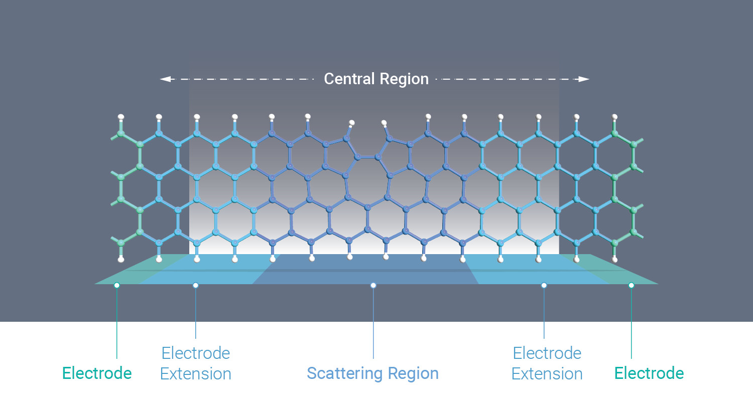
Current may flow between the two bulk Electrodes, but has to pass through the Scattering Region in the middle of the device. Both ends of the central region, called the Electrode Extensions, must be exact replicas of the corresponding electrode.
Graphene Nanoribbon Device
The tutorial section Building a Graphene Nanoribbon Device teaches you how to build the
graphene nanoribbon device used here. In this tutorial you should simply use a device
configuration that is already prepared for you: nanoribbon.hdf5.
Download this file, and note where it is saved.
Start up QuantumATK, open the
project named “Example Project”, go to and locate
the downloaded HDF5 data file nanoribbon.hdf5. Select it and click Open.
Now locate the file in the Project Files list.
Make sure the file is ticked and then follow these steps:
On the LabFloor, select the
 DeviceConfiguration item
saved in the HDF5 file.
DeviceConfiguration item
saved in the HDF5 file.A calculation was already done for this device. Use the General Info tool to see some of the parameters used for the calculation.
Finally, use the
 Viewer to visualize the graphene nanoribbon device. Note the
defect in the middle of the central region, and that both electrodes consist of
pristine (non-defected) nanoribbon unit cells.
Viewer to visualize the graphene nanoribbon device. Note the
defect in the middle of the central region, and that both electrodes consist of
pristine (non-defected) nanoribbon unit cells.
Important
The C-vector of the device configuration simulation cell is aligned with the Z-axis, which in QuantumATK is the transport direction. The left/right electrodes may be different, but must both be periodic in the transport direction. The central (scattering) region is semi-infinite in the transport direction, where it couples to the electrode leads.
Transport Analysis
IV Characteristics
The IV Characteristics study object is a main QuantumATK electron transport analysis tool: It calculates I–V curves from finite-bias transmission spectra, and offers a range of additional analysis methods. The HDF5 file already contains the pre-calculated data, so select the IVCharacteristics object on the LabFloor and open the IV-Characteristics Analyzer tool to analyze it.
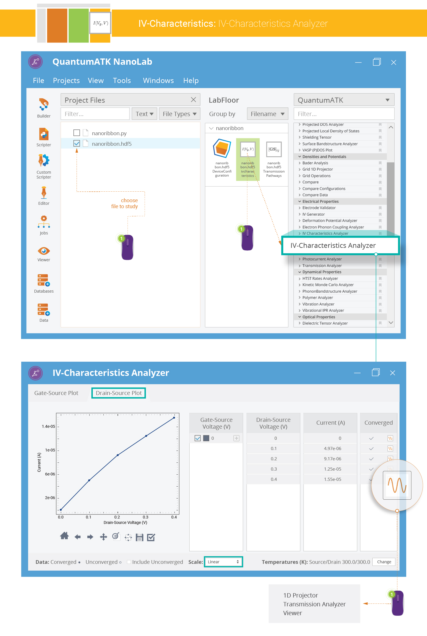
Select the Drain-Source Plot and choose a linear scale for the plot of drain-source current vs. drain-source bias voltage.
The current and simulation convergence status for all sampled bias points are shown in the table. By clicking the plot icon next to a voltage in the table, analysis may be carried out for that particular bias, for example visualization of the corresponding transmission spectrum.
Transmission spectrum
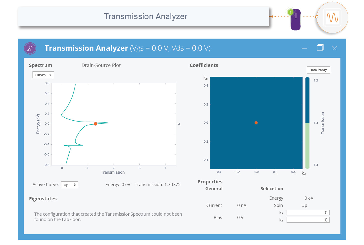
Investigate next the electronic transmission spectrum at zero bias voltage.
Open the Transmission Analyzer by clicking the icon  in the zero-bias row in the table shown in the IV-Characteristics Analyzer
(see image above). The Transmission Anaæyzer will open, as illustrated below.
in the zero-bias row in the table shown in the IV-Characteristics Analyzer
(see image above). The Transmission Anaæyzer will open, as illustrated below.
The left-hand plot shows the transmission spectrum (electron energy vs. transmission), while the right-hand plot shows an interpolated contour plot of the transmission coefficients in reciprocal space.
Transmission eigenstates
For a given energy and k-point, the electron transport can be described in terms of transmission eigenstates. QuantumATK has a separate analysis object for this, named TransmissionEigenstates.
In this tutorial, the zero-bias transmission eigenstates for quantum numbers 0, 1, and 2 were already calculated as an additaional analysis on the IV Characteristics study object. These three eigenstates can therefore be visualized from the IV-Characteristics Analyzer.
Return to the IV-Characteristics Analyzer window and click the zero-bias
icon, then click Viewer to visualize the transmission eigenstates.
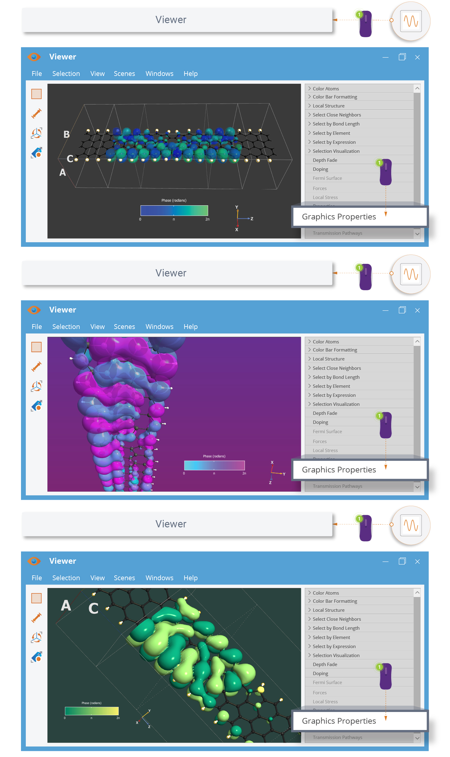
A dialog asks how you want to visualize the eigenstates – select
isosurface. In the Viewer window that pops up,
open the Properties menu, and set the isovalue to 0.1 for each isosurface.
You will then see the following visualizations of
the transmission eigenstates through the graphene nanoribbon device.
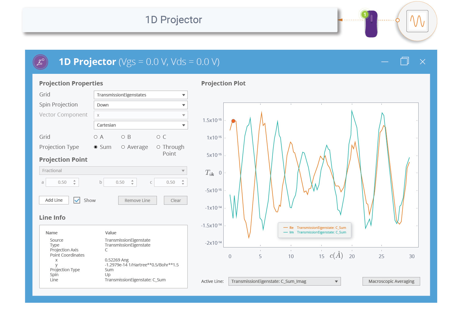
The 1D Projector is also available as an alternative visualization method. As illustrated below, by projecting the transmission eigenstates grid quantities onto a single real-space axis, the eigenstates may be visualized in a 2D plot.
Transmission Pathways
Finally, you should calculate the zero-bias transmission pathways at the Fermi level.
This allows you to visualize the pathways for electron transmission from the
left to the right electrode. Load the DeviceConfiguration stored in the
nanoribbon.hdf5 data file.
Make sure the analysis script saves output data to pathways.hdf5,
and save the analysis script as pathways.py.
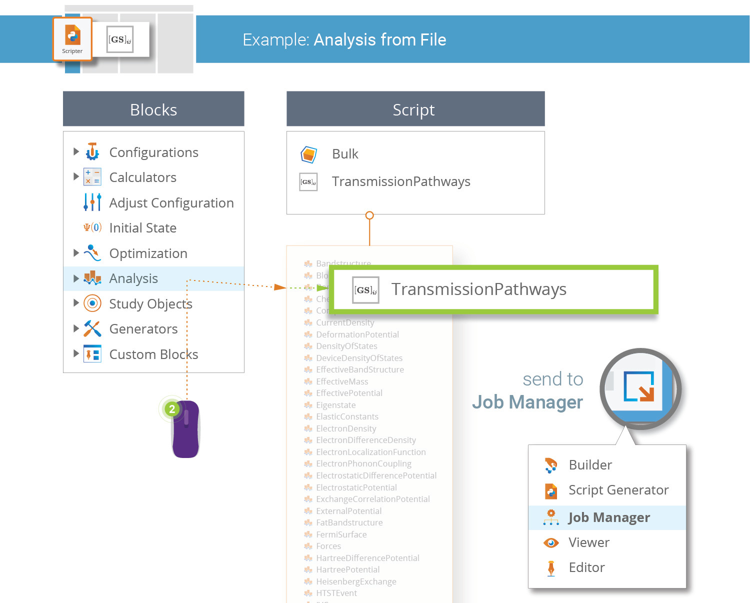
The TransmissionsPathways data item,  , should now be
available on the LabFloor. Visualize it using the Viewer, as illustrated
below. The volume of each arrow indicates the magnitude of the local transmission
between each pair of atoms, while the arrow and color indicate the direction of
the electron flow.
, should now be
available on the LabFloor. Visualize it using the Viewer, as illustrated
below. The volume of each arrow indicates the magnitude of the local transmission
between each pair of atoms, while the arrow and color indicate the direction of
the electron flow.
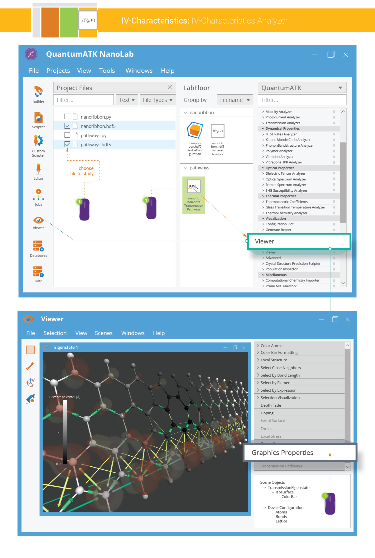
It is not hard to deduce the positions of the atoms, but you can also add them
explicitly by dropping the DeviceConfiguration
onto the  Viewer canvas.
However, the bonds hide the arrows, so you may want to adjust the radius of the atoms.
Use the Properties menu for this.
Viewer canvas.
However, the bonds hide the arrows, so you may want to adjust the radius of the atoms.
Use the Properties menu for this.
Performing the Device Calculations
The transport analysis in the previous section was done using pre-calculated data. However, it is fairly simple for you to redo the device simulation and compute the I-V curve on your own. Just follow the instructions given below.
On the LabFloor, select the DeviceConfiguration
previously saved in the nanoribbon.hdf5 data file. Drop it
on the Scripter and notice that both the device
configuration and saved calculator are added to the script.
Then add the IVCharacteristics block to the script,
and set the default output filename.
Tip
You can use the mouse to reorder the inserted script blocks if needed. You can also delete blocks using Delete on your keyboard.
Next, you should make sure that each script block is set up properly:
Double-click the
 Calculator block to open it and check the
calculator parameters. In particular, make sure to use the Extended Hückel semi-empirical method.
Calculator block to open it and check the
calculator parameters. In particular, make sure to use the Extended Hückel semi-empirical method.Moreover, the calculator density mesh cut-off should be 20 Hartree, and the Cerda.Carbon[graphite] basis set should be used for carbon.
No options should be changed in the IVCharacteristics block, but you should open it to see the available options.
Additional analysis of the transmission eigenstates may be manually added to the IV Characteristics block. To do this, send the script to the
 Editor and insert at the bottom the script lines given below.
# -------------------------------------------------------------
# TransmissionEigenstate analysis for quantum numbers [0,1,2]
# -------------------------------------------------------------
for i in [0,1,2]:
    iv_characteristics.addAnalysis(
        0.0 * Volt,
        0.0 * Volt,
        TransmissionEigenstate,
        {'quantum_number': i}
        )

# Update IV characteristics again.
iv_characteristics.update()
Remember to save the script, and perhaps compare your result to
nanoribbon.py.
You are now ready to run the calculations – you can use the  Job Manager for this. Please note that the job may take several hours if run in serial on a
standard desktop computer. You may bring this down to less than an hour if you
run the job in parallel on multiple computing cores, either on your local machine or on a
remote computing cluster.
Job Manager for this. Please note that the job may take several hours if run in serial on a
standard desktop computer. You may bring this down to less than an hour if you
run the job in parallel on multiple computing cores, either on your local machine or on a
remote computing cluster.